Last year I built a football betting model (algorithm) in Python to help me make data-driven predictions and to identify betting opportunities in the English Premier League (EPL).
Predicting Football With Python
This year I re-built the system from the ground up to find betting opportunities across six different leagues (EPL, La Liga, Bundesliga, Ligue 1, Serie A and RFPL).
After completing my last model in late December 2019 I began putting it to the test with £25 of bets every week. Unfortunately, I only managed to fit in eight weeks of betting before COVID-19 cut the EPL short.
The good news is that I broke even during this period, I bet £200 and I got £200 back.
But I'm not here to break even.
In this article I'm going to explain my methodology, technical implementation and betting strategy in order to help you create your own betting model with Python. This can then be then used to assist you in making the right choices when betting on the Bundesliga at one of the top German betting sites.
A good betting strategy can become the key to success if it is applied correctly.
But one must be careful to pick the right company. You can look at Bet365 India as an example of a reliable online bookmaker.
Their desktop platform and mobile app are both user-friendly and allow you access to a wide array of their services. They offer a chance to get profit by online betting. You can go to Sportsbook Review & Rating and check it out yourself.
Methodology & Code
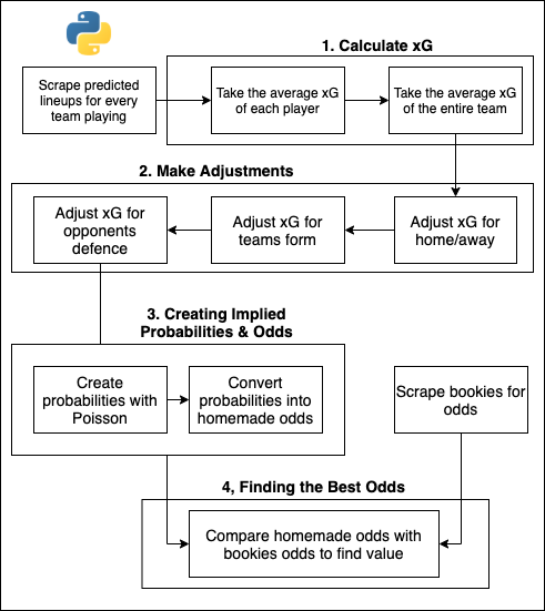
The new model leverages a lot of the code that was used in the previous model and can be simplified into four steps:
- Calculate the average expected goals of every team
- Adjust this value based on form, home/away and the oppositions defensive score
- Convert this adjusted average value for expected goals into implied probabilities and odds for over/under bets
- Compare these odds with the best odds offered by the bookies for overs/unders and make bets based on the likelihood of the outcome

1. Expected Goals
"Expected goals" (xG) is a much better reflection of a team's performance than shots or shots on target. Instead of considering every "shot on target" equally, xG considers the quality of each shot taken by looking at where it was taken, what foot it was taken with and the "style of play".
If you're interested in learning more about this revolutionary metric, I talk about it more in this article: Modern Football Statistics
This step considers the predicted line-ups of each team and looks at their individual xG values over the last n (usually 6) games. I've previously taken the lineups from Fantasy Football Scout:
How to Scrape Predicted Lineups from Fantasy Football Scout with Python
But in order to gather lineups from leagues all over the world I have to scrape lineups from a website that covers games all over the world!
I take the HTML for every fixture in a given season:
html = requests.get(f"https:/X/leagues?id={league_id}&type=league")\
all_season_fixtures = [x["pageUrl"] for x in html.json()["fixtures"]]
Then I get every fixture ID from this list that is in the current game week (current_fixtures pulled from API Football):
final_fixture_ids = []\
for fixture in all_season_fixtures:\
    if fixture.split('/')[4] in current_fixtures:\
        final_fixture_ids.append(fixture.split('/')[2])
I pull the HTML from every fixture:
for fixture in final_fixture_ids:\
    url = https:/X/?matchId={fixture}'\
    data = requests.get(url, headers=headers, allow_redirects=False).json()\
    lineups.update(parse_lineups(data))
And I parse the HTML:
def parse_lineups(raw_data: Dict) -> Dict:\
    lineups = {}\
    for team in raw_data['content']['lineup']['lineup']:\
        team_name = team['teamName']\
        lineup = {}\
        for positions in team['players']:\
            for player in positions:\
                lineup[player['name']] = player['id']\
        lineups[team_name] = lineup\
    return lineups
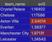
The program then sums every players average expected goals (avG) from a database of player attributes and divides it by the number of players (11). In other words, it's the average expected goals for the entire team over a given period.

This feature was written under the assumption that betting markets become more efficient as the event draws nearer. Because as more bets are made, the "Wisdom of the Crowd" effect takes over (collective opinion is more accurate than one expert opinion). That's why I make all of my bets well in advance of the games with the predicted lineups.
2. Adjustments
Once xG has been calculated for every team that's playing on a given day, the following adjustments are made:
Home/away: I assume that teams who are playing at home are expected to score 10% more goals on average, whilst teams who are playing away will score 5% less on average.
for fixture in fixtures:

    df.loc[df['team_name'] == fixture['homeTeam']['team_name'], 'home_away_adjustment'] = master_params()['HOME_ADVANTAGE']

    df.loc[df['team_name'] == fixture['awayTeam']['team_name'], 'home_away_adjustment'] = master_params()['AWAY_ADVANTAGE']

df['avG_adjusted'] = df.av_xG * df.home_away_adjustment
Defence of Opposition: By comparing the opposition's previous xG with their actual goals scored in a game, I create a "defence factor" which I use to adjust their average xG. E.g. if a team had an xG of 2.35 and they only scored one goal then the opposition must have defended well.
for result in recent_results:
xG_diff = float(result['xG'][opponents_side]) - float(result['goals'][opponents_side])
xG_diff_total = xG_diff_total + xG_diff
xG_diff_avg = xG_diff_total / fixture_history
Form: This adjustment considers how many of the last n games the team has won/drawn/lost when playing at home or away. It also considers their recent "streak", whether that be a streak of wins, draws, or losses.
# Home side wins\
if fixture['goalsHomeTeam'] > fixture['goalsAwayTeam']:\
    if fixture['awayTeam']['team_name'] in list(df_team.index.values):\
        update_dataframe('a', 'loss', df_team, fixture)\
    elif fixture['homeTeam']['team_name'] in list(df_team.index.values):\
        update_dataframe('h', 'win', df_team, fixture)
This creates the final dataframe before calculating probabilities and odds.

3. Creating Implied Probabilities & Odds
Now that we have a team's average expected goals for a given game, we can put this into Poisson's distribution.

Poisson distribution (Lambda = average value over given time, k = number of events e.g. goals)
for goals_scored in range(largest_goals_scored):\
    for team in teams:\
        avG = df_Poisson.at[goals_scored, team]\
        df_Poisson.at[goals_scored, team] = ((math.exp(-avG) * math.pow(avG, goals_scored)) / math.factorial(goals_scored))
This equation is a discrete probability distribution that predicts the probability of discrete events over a fixed time interval (e.g. goals scored over ninety minutes).

I make the assumption that because scoring more than five goals is so unlikely in a given game, I only calculate the probabilities of zero to five goals (although this season is FILLED with goals). So now we've got every team's probabilities for scoring goals, it's time to create our own odds.
3.5 Creating 'Homemade' Odds
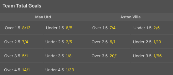
My betting strategy currently focuses on "over and under" bets, which are concerned with teams scoring over x or under y amount of goals. E.g. I bet that Manchester United will score over two goals against Aston Villa.

In order to work out the probabilities of these events, I simply take the sum of probabilities for a team scoring that many goals or more.
E.g. for "over 1.5" goals I would sum the probabilities of a team scoring 2, 3, 4 and 5 goals.
df_implied_probability.at[team, 'O1_5'] = df.at[team, '2'] + df.at[team, '3'] + df.at[team, '4'] + df.at[team, '5']
Odds are simply the inverse of implied probabilities, so inverting this number provides me with my very own homemade odds for "overs and unders"!

I've gone over some of the code that I used to create these dataframes in a previous article if you're interested:
Betting on Football With Python
4. Finding the Best Odds & Strategy
After calculating my own complete set of odds, the program then proceeds to scrape data from over twenty betting websites. It returns the best odds for each betting market that I'm interested in along with the names of the associated UK online bookmakers.
This data is formatted in exactly the same way as my previous dataframe so that I end up with this:

In order to find "value" bets (where I believe a bookmaker has predicted an outcome to be more unlikely than I believe it to be) I need to find the difference between the bookies odds and my homemade odds :
df_betting_alpha = df_bookies_odds - df_over_unders
When values within my "df_betting_alpha" dataframe are positive then this implies that there is "value" in that bet, because the bookies are better odds than my homemade odds imply:

The difference between the bookies odds and homemade odds (alpha) for each team in game week 15 (27.12.2020)
So when the bookies odds are higher than the homemade odds, that implies that this is potentially a good bet to make. In the above picture the model correctly identified that betting on Liverpool to not score as many goals as usual would've been a profitable bet to make (U1_5 & U2_5).

4.5 Betting Strategy
Once the program has all of these dataframes, there is a final stage of analysis to help identify the most profitable bets.
For each bet that could potentially be made, there are three threshold values that need to be exceeded in order for the bet to be made:
- Alpha Threshold: The bookies must have under-predicted this outcome by a given amount.
- Homemade Odds Threshold: The minimum homemade probability of an outcome.
- Bookies Odds Threshold: The minimum probability of an outcome provided by the bookies. This also implies a minimum odds that I'm willing to bet on.
These thresholds allow the betting strategy to be adjusted appropriately, it is possible to take on more risk by reducing these values and by making more bets. I've found it more profitable to make a few bets with higher thresholds.
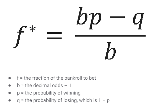
The amount that is placed on each bet is dictated by the Kelly Criterion:

The Kelly Criterion (source)
This formula suggests how much of your total bankroll should be placed on each bet based on the probability of winning that bet.
Saving Data to AWS S3
Every dataframe that has been created during this analysis is automatically uploaded into a datalake (S3) for future analysis. Each row is split out and saved into its own file in order to partition the data by team.
This code snippet demonstrates how to save a dataframe row by row:
for index, row in df.iterrows():\
    single_data_row = {}\
    for series_index, series_value in row.items():\
        single_data_row[series_index] = series_value\
    team = index.replace(' ', '_')\
    csv_buffer = StringIO()\
    headers = list(single_data_row.keys())\
    writer = csv.DictWriter(csv_buffer, fieldnames=headers)\
    writer.writeheader()\
    writer.writerow(single_data_row)\
    filepath = f'data/{season}/overunders/{league_name}/{team}/{current_round_formatted}/{filename}'\
    logger.info(f'Saving to {filepath}')\
    s3_response = s3_resource.Object(s3_bucket, filepath).put(Body=csv_buffer.getvalue())
Conclusion
The algorithm is now capable of making and comparing odds on outcomes across six different football leagues.
Betting opportunities are identified by analysing four metrics (xG, form, home/away and opposition defence) to generate "homemade" odds which are then compared against the best odds offered by the bookies.
Expanding this algorithm across six different leagues allows more betting opportunities to be identified throughout the season.
In the future I'm going to create a database which will allow backtesting of betting strategies to further optimise this betting process, but for now I'm going to enjoy another season of football!
