Hi everyone, today we are going to talk about one of the best and most famous search algorithms, the well-known A* Algorithm. Till now we had the opportunity to study and implement in Python a couple of search algorithms, such as the Breadth-First Search (BFS), the Depth First Search (DFS), the Greedy Algorithm, etc. Today we are closing the chapter with Search Algorithms talking about the A*. More specifically, we will talk about the following topics:
1. Introduction
2. Pseudocode
3. Pen and Paper Example
4. Python implementation
5. Example
6. Conclusion
As usual, we have a lot of stuff to cover, so let's get started.
Introduction
As we have already discussed, search algorithms are used to find a solution to a problem that can be modeled into a graph.
If you want to learn more about Graphs and how to model a problem, please read the related article.
In brief, a graph consists of a set of nodes (or vertices) and edges that connect the nodes. Each state (situation) of the given problem is modeled as a node in the graph, and each valid action that drives us from one state to another state is modeled as an edge, between the corresponding nodes.
In these problems, we know the starting point (initial state — node) and we have a target (state — node), but we probably do not know how to approach the target, or we want to achieve it in an optimal way.
Search Algorithms start from the initial state (node) and following an algorithmic procedure search for a solution in the graph (search space). Graph Data Structure — Theory and Python Implementation
Search Algorithms are divided into two main categories. The first category contains the so-called “blind” algorithms.
These algorithms don't take into account the cost between the nodes. Breadth-First Search and Depth First Search algorithms are characterized as “blind”.
On the other hand, the algorithms in the second category execute a heuristic search, taking into account the cost of the path or other heuristics.
The latter category belongs to the Greedy algorithm and the USC algorithm we talked about in previous articles. Α* is also a heuristic algorithm.
Pseudocode
The A* algorithm runs more or less like the Greedy and the UCS algorithm. As you probably remember, the heuristic function of the Greedy Algorithm tries to estimate the cost from the current node to the final node (destination) using distance metrics such as the Manhattan distance, the *Euclidean distance*, etc.
Based on this value the algorithm determines the next selected node. On the other hand, the heuristic function of the UCS algorithm calculates the distance of the current node from the start node (initial state — node) and selects as the next node the node with the smallest value, or in other words the node closer to the initial node.
A* algorithm combines these two approaches, using a heuristic function that calculates the distance of the current node from the initial node and tries to estimate the distance from the current node to the target node, using for example the Manhattan distance. The sum of these two values is the heuristic value of the nodes, determining the next selected node.
The A* algorithm takes a graph as an input along with the starting and the destination point and returns a path if exists, not necessarily the optimum.
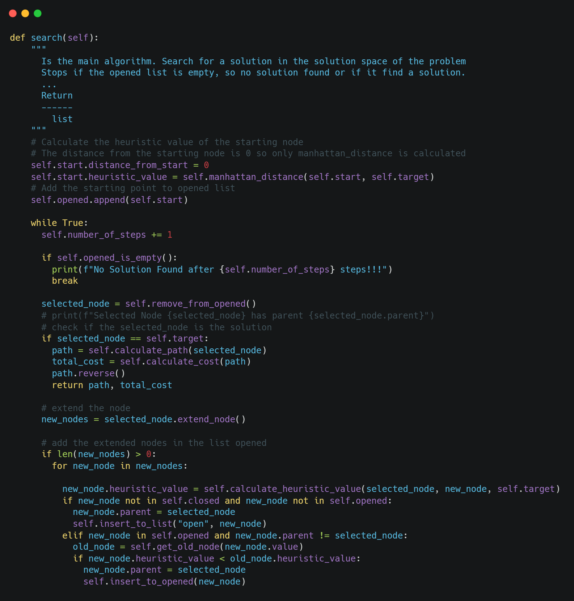
To do that it uses two lists, called *opened *and closed. Opened list contains the nodes that are possible to be selected and the closed contains the nodes that have already been selected. Firstly, the algorithm calculates the heuristic value of the first node, and append that node in the opened list (initialization phase).
After that, remove the initial node from the opened list put it on the closed list. Next, the algorithm extends the children of the selected node and calculates the heuristic value of each one of them. If a child does not exist in both lists or is in the opened list but with a bigger heuristic value, then the corresponding child is appended in the opened list in the position of the corresponding node with the higher heuristic value. Otherwise, it is omitted.
In each step, the node with the minimum heuristic value is selected and be removed from the opened list.
The whole process is terminated when a solution is found, or the opened list is empty, meaning that there is not a possible solution to the related problem.
The pseudocode of the A* algorithm is the following:
    function Greedy(Graph, start, target):
        calculate the heurisitc value h(v) of starting node
        add the node to the opened list
        while True:
            if opened is empty:
            break # No solution found
            selecte_node = remove from opened list, the node with
                        the minimun heuristic value
            if selected_node == target:
               calculate path
               return path
            add selected_node to closed list
            new_nodes = get the children of selected_node
            if the selected node has children:
               for each child in children:
                  calculate the heuristic value of child
                  if child not in closed and opened lists:
                     child.parent = selected_node
                     add the child to opened list
                  else if child in opened list:
                     if the heuristic values of child is lower than                the corresponding node in opened list:
                        child.parent = selected_node
                        add the child to opened list where h(v) is the sum of the distance of the v node from the initial node and the estimated cost from v node to the final node.
Pen and Paper Example
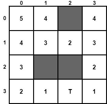
To better understand the A* algorithm, we are going to run an example by hand. We will use the same example we used in the article about the Greedy algorithm, with the difference that now we will use weights on the edges of the graph. So, we have the following maze:

Suppose we have a robot and we want the robot to navigate from point S in position (0, 0) to point T in position (3, 2). The grey squares are obstacles that cannot pass the robot. To find a path from point A to point T, we are going to use the Greedy Algorithm. As a heuristic function, we will use the Manhattan Distance. Thus, we are going to calculate the Manhattan Distance of all the cells of the maze, using the following formula.
manhattan((x1, y1), (x2, y2)) = |x1 — x2| + |y1 — y2|
We first calculate the Manhattan distance for all the cells of the maze. The corresponding distances are the following:
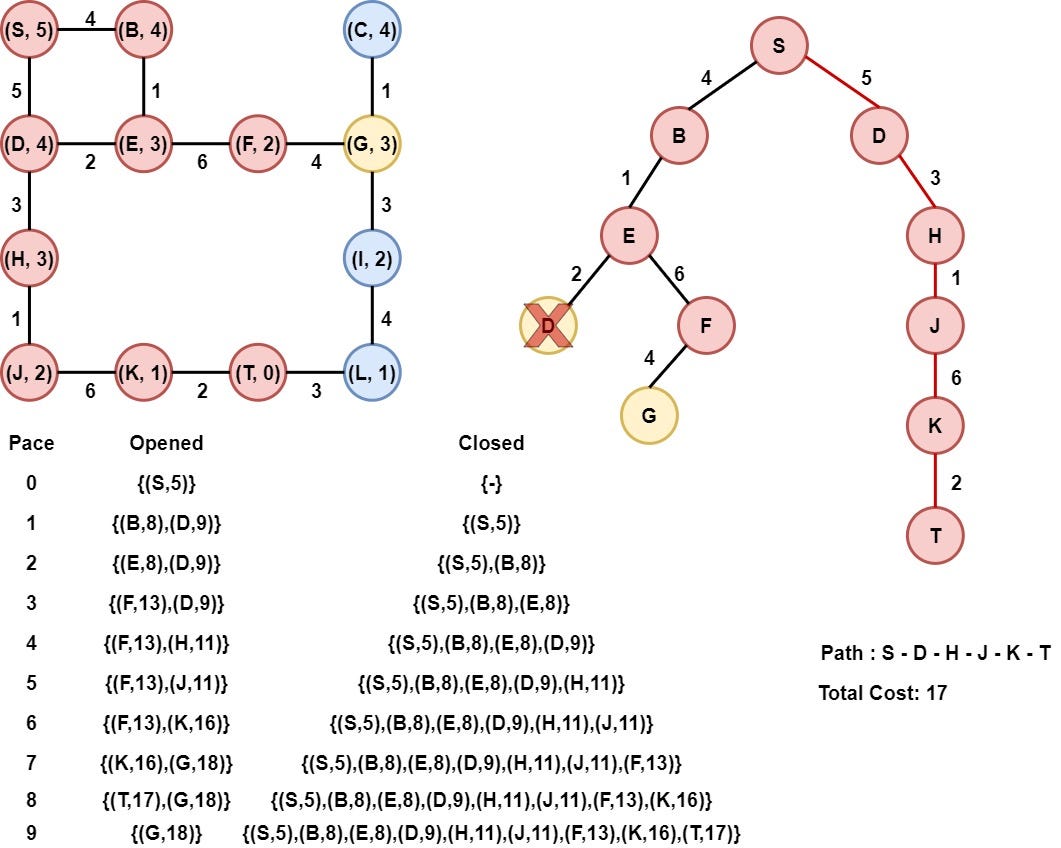
Now, we are ready to turn (model) the above maze into a graph. So we have the following graph:
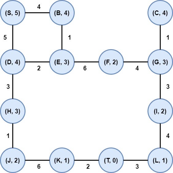
Notice that we have inserted weights in each edge that represents the necessary energy for the robot to go from one node to another. Moreover, inside of each node, we have noted the manhattan distance. Now, we are ready to execute the A* algorithm.
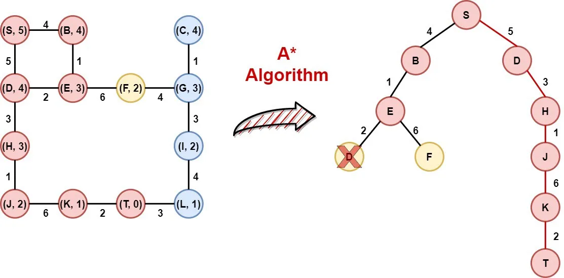
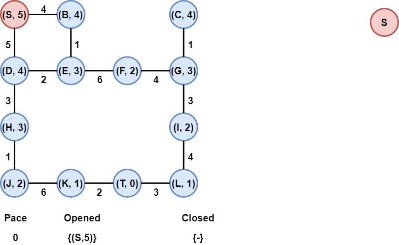
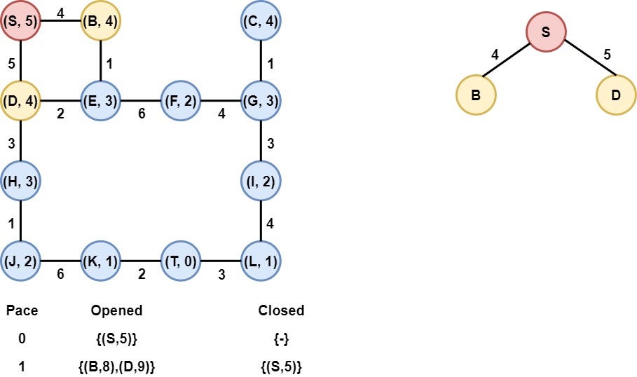
Step 1: Initialization
We put the node in the opened list after evaluating its heuristic value.
Step 2: Node S in selected
Node S is removed from the opened list and is added to the closed list. Moreover, the children of S, nodes B, D are added to the opened list after the calculation of their heuristic values.
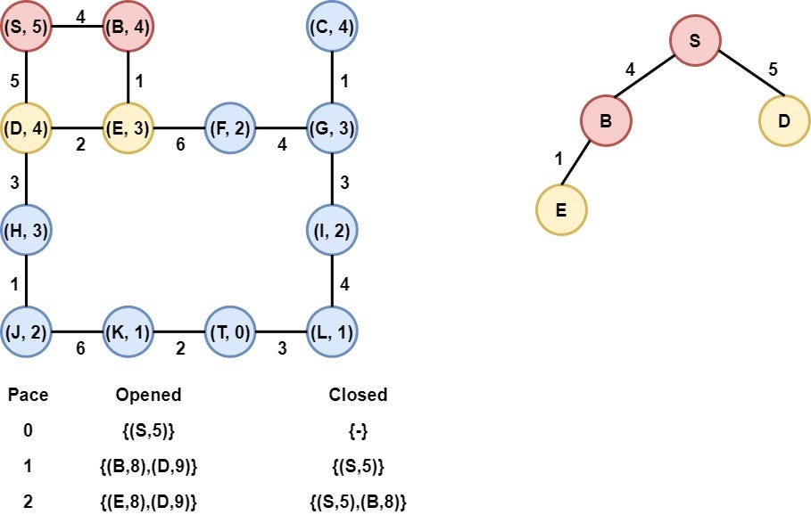
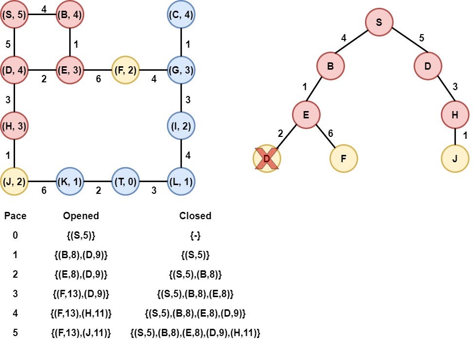
Step 3: Node B is selected
Node B is selected as it has the smallest heuristic value. Node B is removed from the opened list and is added to the Closed list. After that, the heuristic value of its child (Node E) is calculated and node E is appended to the opened list.
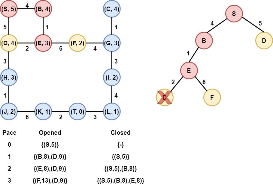
Step 4: Node E is selected
Node E is selected as it has the smallest heuristic value. Node E is removed from the opened list and is added to the Closed list. After that, the heuristic value of its children(Nodes D and F) are calculated and node F is appended to the opened list. On the other hand, node D is already in the opened list with a heuristic value equal to 9, the new heuristic value of node D is 11, which means is bigger and thus we keep the old node D (with the node S as its parent) in the opened list.
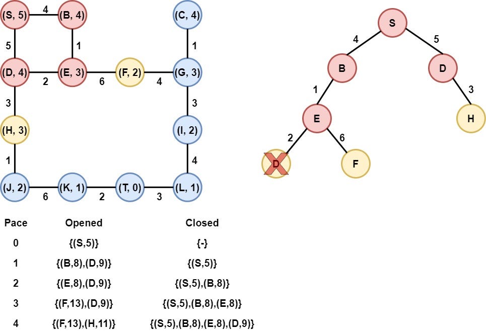
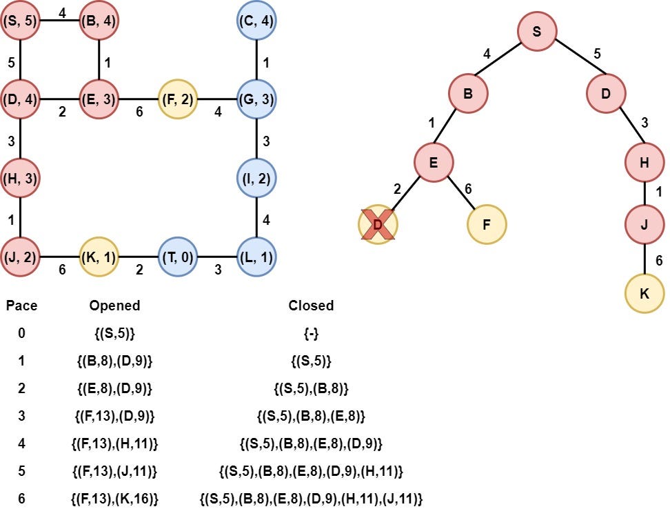
Step 5: Node D is selected
Node D is selected as it has the smallest heuristic value. Node D is removed from the opened list and is added to the Closed list. After that, the heuristic value of its children(Nodes E and H) are calculated and node E is appended to the opened list. On the other hand, node E is already in the closed list, thus it is omitted.
Step 6: Node H is selected
Node H is selected as it has the smallest heuristic value. Node H is removed from the opened list and is added to the Closed list. After that, the heuristic value of its child(Node J) is calculated, and node J is appended to the opened list.
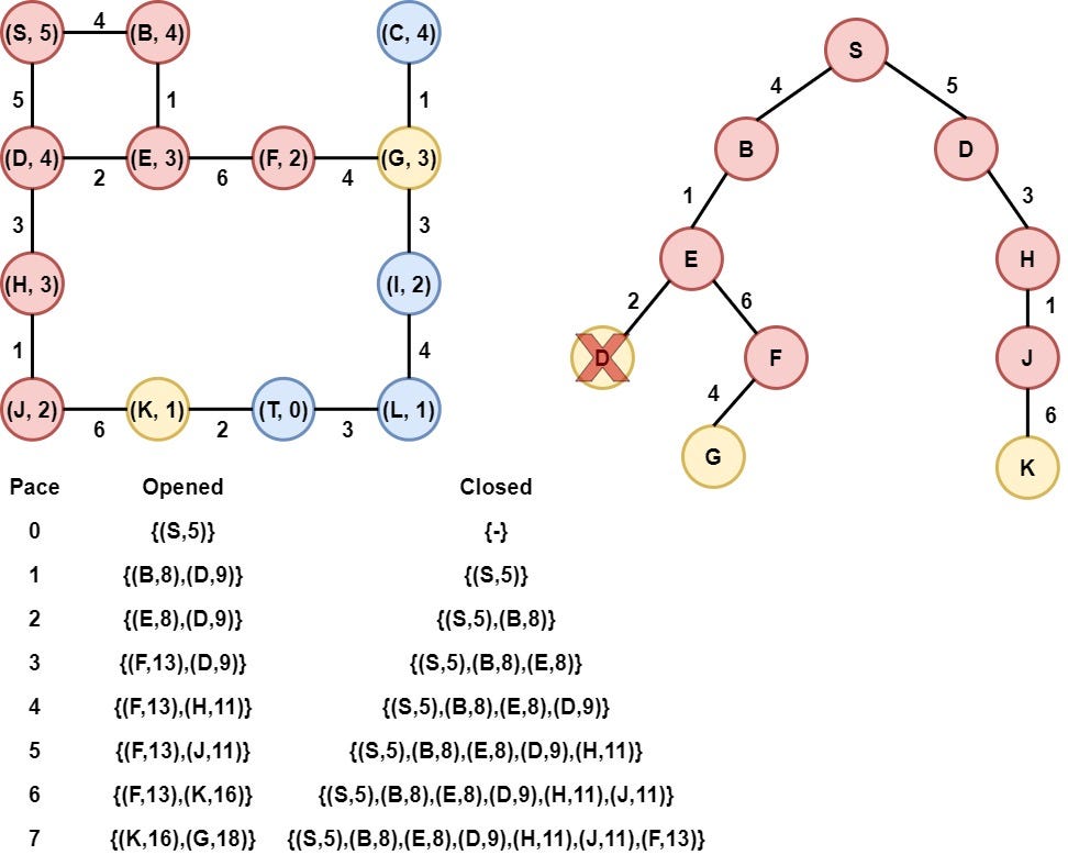
Step 7: Node J is selected
Node J is selected as it has the smallest heuristic value. Node J is removed from the opened list and is added to the Closed list. After that, the heuristic value of its child(Node K) is calculated, and node K is appended to the opened list.
Step 8: Node F is selected
Node F is selected as it has the smallest heuristic value. Node F is removed from the opened list and is added to the Closed list. After that, the heuristic value of its child(Node G) is calculated, and node G is appended to the opened list.
Step 9: Node K is selected
Node K is selected as it has the smallest heuristic value. Node K is removed from the opened list and is added to the Closed list. After that, the heuristic value of its child(Node T) is calculated, and node T is appended to the opened list.
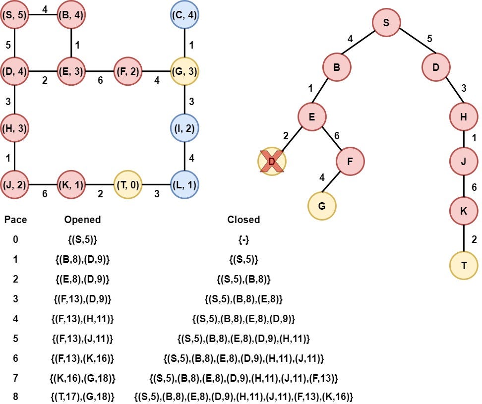
Step 10: Node T is selected
Node T is selected as it has the smallest heuristic value. Node T is the target node, so the algorithmic procedure is terminated and is returned the path from node S to node T, along with the total cost.
Python implementation
Having understood how the A* algorithm works, it is time to implement it in Python.
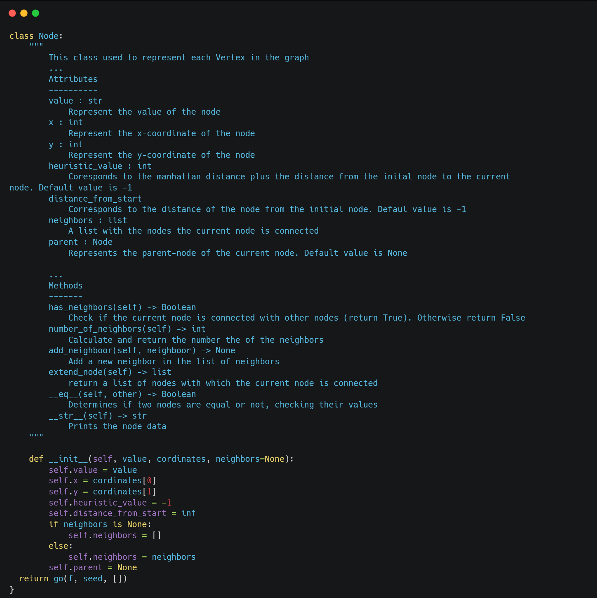
Firstly, we create the class Node that represents each node (vertex) of the graph. This class has a couple of attributes, such as the coordinates x and y, the heuristic value, the* distance from the starting node*, etc. Moreover, this class is equipped with methods that help us to interact with the nodes of the graph. In the following image, we have an overview of the class.
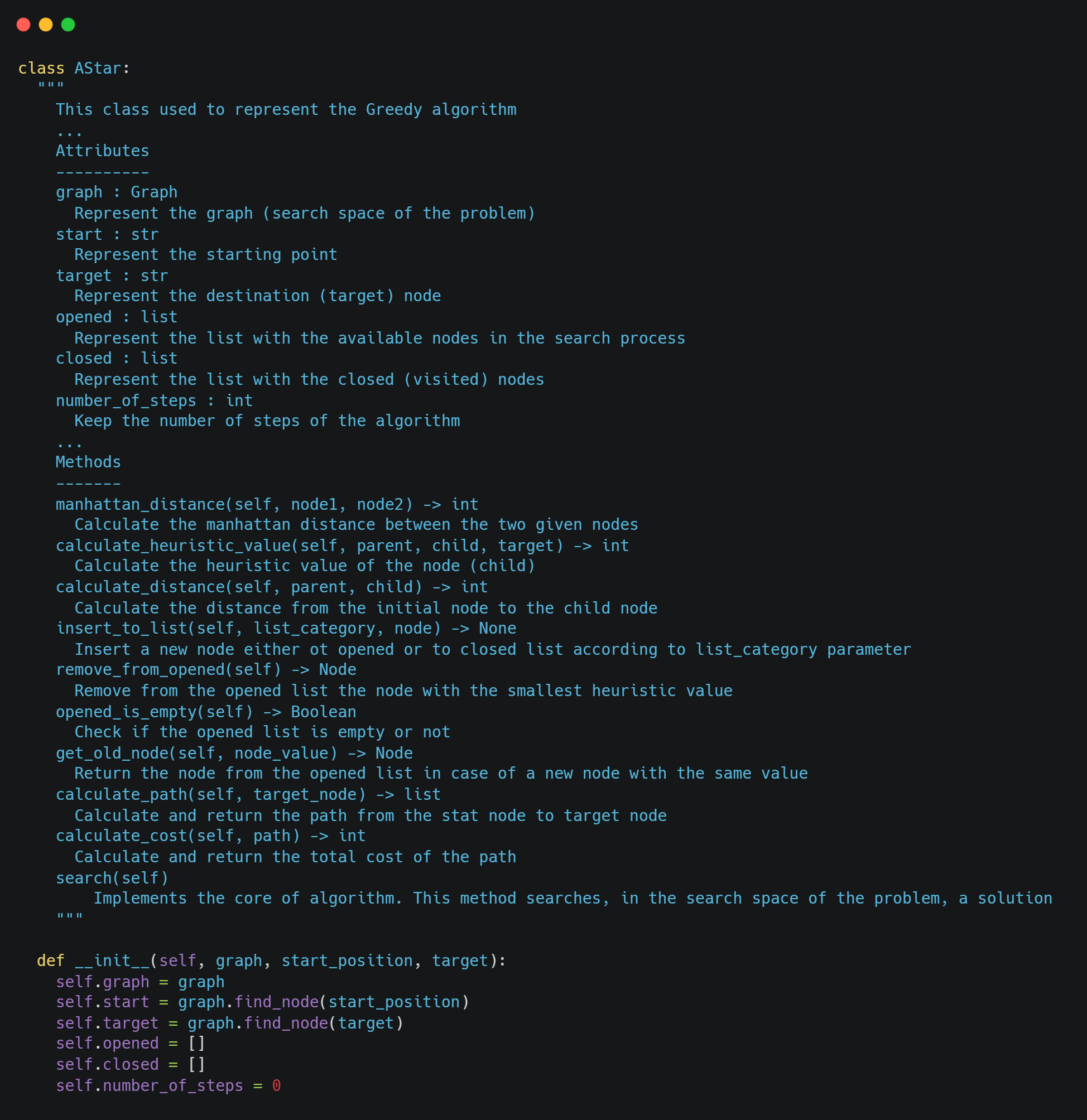
After that, we implement the class AStar, which represents the algorithm. The class AStar has a couple of attributes, such as the _graph _(search space of the problem), the starting point, the target point, the opened and closed list, etc. An overview of the class is the following:
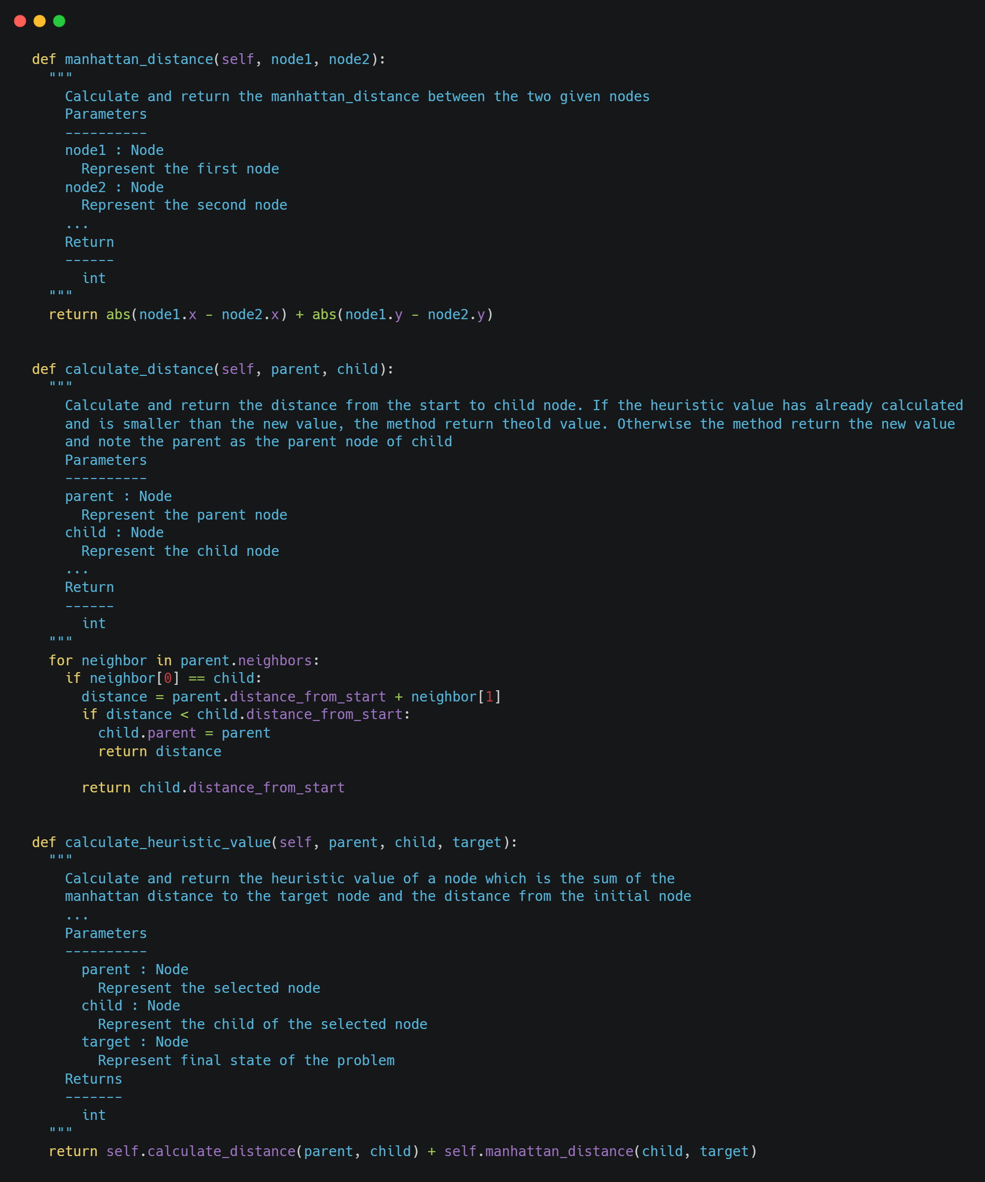
To calculate the heuristic value, we add the manhattan distance with the distance from the initial node. An overview of these functions is the following:
Finally, the core algorithm is the following
Example
Now, we have the algorithm and we are able to execute the A* algorithm in any graph problem. We are going to check the algorithm in the example above. The graph is the following:
so we will model the above graph as follows and we will execute the algorithm.
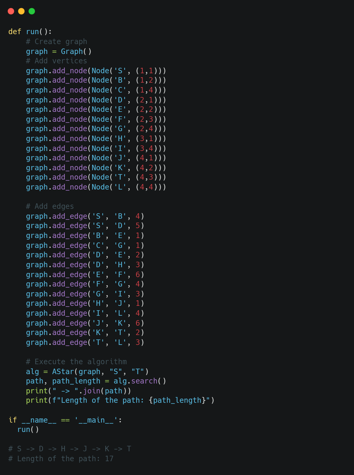
We can notice that we got the same results. Remember that the A* algorithm always returns the optimal solution.
You can see and download the whole code here.
Conclusion
In this article, we had the opportunity to talk about the A* algorithm, to find the optimum path from the initial node to the target node. A* algorithm, just like the Greedy and the USC algorithms uses a heuristic value to determine the next step. Moreover, the A* algorithm always returns the optimal solution. With the A* we have finished with the search algorithms. In the future, we will have the opportunity to compare all of them using the same data, visualizing the whole algorithmic process. Until then, keep learning and keep coding. Thanks for reading.
Learn more about Search Αlgorithms. Solve Maze Using Breadth-First Search (BFS) Algorithm in Python
How to Solve Sudoku with Depth-first Search Algorithm (DFS) in Python
Comments
Loading comments…