A stock’s beta measures how risky, or volatile, a stock’s price is compared to the entire market. When beta is less than 1, a stock is less volatile, or less risky than the market. The opposite holds true when beta is greater than 1, showing the stock would be more volatile, or riskier than the market. A beta equal to 1 represents a stock that has equal risk and volatility as the market.
Stock betas are provided to investors by brokerage firms such as Fidelity or Schwab, or by financial sites like Yahoo Finance. The problem is, if you were to visit three different online sites, you would likely get three different betas for the same stock.
Below is the beta for American Express (AMX) as of February 22, 2021, from three leading financial entities:
- Fidelity: 1.73
- Schwab: 1.31
- Yahoo Finance: 1.28
The differences come from the way each site calculates the beta. One site may use monthly prices for 3-years. Another may use monthly prices for 5-years, while another may define the ‘market’ differently and choose a different comparison variable.
Few investors buy and hold a stock for 3 to 5 years anymore. Many people trade stocks daily or may hold them for a short period before selling them. Knowing how a stock reacts over a 5-year time frame holds little value for that type of investor.
In the model shown in this article, we are going to solve for the 1 year beta of the American Express Company (AXP). As an investor, you should have the ability to choose how you want to assign the beta to your investments.
A short-term investor faces two major questions concerning stock risk:
- What is the real beta when the professionals say the range is between 1.28 and 1.73?
- My investment time horizon is a year or less. Not 3 to 5 years, so is that beta range even applicable?
How a Stock’s Beta is Measured
There are two methods available to measure a stock’s beta. Both are expected to result in the same numerical outcome.
- Beta = Covariance / Variance: Where covariance is the stock’s return relative to the market's return. Variance shows how the stock moves in relation to the market. We used covariance to determine if the market and American Express moved in the same direction today. Variance would see if American Express and the market moved the same amount. If the market went up 0.5% today, did American Express also go up 0.5%? Or did it go up by less than 0.5% or by more than 0.5%?
- Beta: y= a + (b*x): Another way to calculate beta is to use a linear regression formula. Where beta is the coefficient of the independent variable (x in the equation), y is the dependent variable, a is the y-intercept or constant, and b is the slope of the line.
Since both measurements provide us with the same answer, this article will outline how to use the regression formula y = a + (b * x) where x is the beta.
Why?
Because creating regression models in python is easier, and can be accomplished with a few lines of code. Calculating covariances and variances can be done in python but requires extra steps.
Load Historical Stock Price Data
In Python, start out by loading the following libraries:
- Yfinance will get the stock prices.
- Numpy to manipulate data.
- Sklearn.linear_model will be used for the linear regression.
import yfinance as yf
import numpy as np
from sklearn.linear_model import LinearRegression
Next, create a list of “symbols” that will hold both the stock symbol for the beta model and the market symbol for comparison.
# symbols = [stock, market]
symbols = ['AXP', 'SPY']
In the above example, the symbol ‘AXP’ represents American Express. The symbol ‘SPY’ represents the S&P 500 ETF Trust, which many people use as a surrogate for the total market. For the rest of this example, we will use ‘SPY’ as a representation of the market. To substitute a different market surrogate, instead of ‘SPY’, choose the symbol you want instead. As long as yfinance has the data, you can use the model to calculate international stocks. Select the stock from the country you want, then substitute the market index ‘SPY’ for the equivalent market index in the home country of the selected stock. Other than the symbol changes, no other changes are necessary.
Creating a Dataframe of Historical Prices
Once the stock and market are selected, load the symbols list into a yf.download() function to create a dataframe of historical stock prices.
# Create a dataframe of historical stock prices
# Enter dates as yyyy-mm-dd or yyyy-m-dd
# The date entered represents the first historical date prices will
#   be returned
# Highly encouraged to leave 'Adj Close' as is
data = yf.download(symbols, '2020-2-22')['Adj Close']
Choosing a Date Range
Typically, a year suffices to get a very good sample. In statistics, as a general rule, sample sizes equal to or greater than 30 are deemed sufficient and the beta you calculate should be valid.
A baseline recommendation is to use the same date as today, but one year earlier for the date range input. With 5 trading days each week, 52 weeks each year, and allowing for about 10 annual holidays, a year will provide us with over 250 daily closing prices. You can always choose more or fewer days, as long as you choose a range with at least 31 daily closing prices. Further in the article, you will discover we lose a day’s worth of data in our model. 31 daily closing prices would leave us with 30 daily observations.
Using Adjusted Close Prices
Adjusted closing prices are preferred because they are already adjusted for stock splits and dividends. Which is a fancy way of saying using adjusted closing price increases our accuracy and decreases the time required to make calculations.
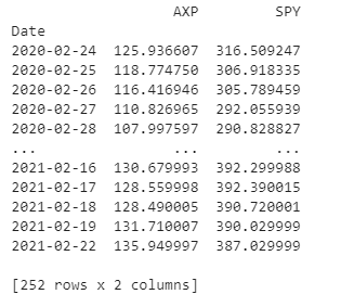
Loading and Viewing Data Table
After running the code, expect to see a loading screen like the one below which shows that the call to yfinance was successfully completed.
Output from JupyterLab:

It is always advisable to review the data you retrieve to make sure it is clean and usable as is and includes the information you were attempting to call. To view the historical data, either print() the entire dataset or use functions such as .head().
# View historical data to confirm it loaded correctly
print(data)
The dates and prices will be different but using the print command on the dataset should produce results similar to the format below.
Output from JupyterLab:
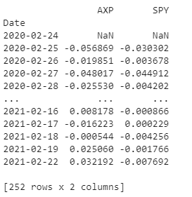
Standardizing Data
The dataset above produces the daily adjusted closing price for both American Express and the S&P 500 surrogate. Since stocks trade at different prices and fluctuate both higher and lower, the measurement must be standardized to show the stock’s movement. Converting the daily adjusted closing prices to a percent change variable is a standardized measure of fluctuation. To do this by hand, we would use the formula ([day2 — day 1] / day 1). In python use, pct_change()
# Convert historical stock prices to daily percent change
price_change = data.pct_change()
print(price_change)
Now, by looking at the dataset, instead of adjusted closing prices, each variable is represented with the daily percent change.
Output from JupyterLab:
Quick Data Cleaning
Pulling directly from the yfinance package creates a very clean dataset. However, when the data was converted from adjusted closing prices to a percent change, the price for the first day creates a NaN value since it is not possible to get a daily price change for the first day.
When using regression to calculate the stock beta, the NaN may produce an error. Therefore, it is best practice to delete the first row that contains the NaN, leaving all the remaining rows containing numbers.
# Deletes row one containing the NaN
df = price_change.drop(price_change.index[0])
Beta Regression Model
Now we are ready to set-up the linear regression model to calculate the stock beta for American Express. Returning to our regression formula where y = a + (b * x), the python LinearRegression() requires two inputs, x and y, where y is the dependent market variable and x is the independent stock variable. Values for a and b are calculated automatically. For sklearn’s LinearRegression() function, the x and y values need to be transformed into NumPy arrays. The x variable has the additional .reshape() added to it as as part of the regression requirement.
# Create arrays for x and y variables in the regression model
x = np.array(df['AXP']).reshape((-1,1))
y = np.array(df['SPY'])
Define the model and set up linear regression as the type of regression.
# Define the model and type of regression
model = LinearRegression().fit(x, y)
The output of our American Express beta model is below. Using this model the beta is 0.403.
# Prints the beta to the screen
print('Beta: ', model.coef_)
with output similar to this:
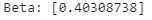
The disparity from our 0.403 from 1.28 to 1.73 range we saw earlier is likely caused by one or more of the following factors: What could cause the large disparity?
- Number of Data Points: In our one-year beta model, we used 251 data points, corresponding to the daily adjusted close price for the past year. The betas provided from the business entities (Fidelity, Schwab, Yahoo Finance) are calculated using month-end prices. This means a 3-year beta would only have 36 data points, while a 5-year beta would only have 60 data points. Typically in statistics, the greater the number of data points translates to a greater level of confidence.
- Recent Risk Profile Change: This past year American Express’s internal risk profile may have changed, becoming less risky compared to the previous three to five years.
- Pandemic Related Changes: Our python model is calculated using historical data from February 2020 to February 2021. Those dates correspond with when the Covid-19 pandemic impacted the stock market. While the models from the financial institutions expand further by including 3 to 5 years.
Finished Product
Below is the code in its entirety (without data confirmation) providing you with a beta in the least time possible.
#load libraries
import yfinance as yf
import numpy as np
from sklearn.linear_model import LinearRegression

# symbols = [stock, market]
# start date for historical prices
symbols = ['AXP', 'SPY']
data = yf.download(symbols, '2020-2-22')['Adj Close']

# Convert historical stock prices to daily percent change
price_change = data.pct_change()

# Deletes row one containing the NaN
df = price_change.drop(price_change.index[0])

# Create arrays for x and y variables in the regression model
# Set up the model and define the type of regression
x = np.array(df['AXP']).reshape((-1,1))
y = np.array(df['SPY'])
model = LinearRegression().fit(x, y)

print('Beta = ', model.coef_)
Conclusion
It only takes a few lines of code to create custom stock beta calculations in Python. When writing your script, a couple of things to remember:
- Enter the stock symbols as a string in all ‘CAPS’
- You only need to change the stock (in 2 places), not the market (i.e. ‘AXP’)
- Change the date (recommend using the same day, 1 year prior)
- You can only run the model on 1 stock at a time.
Thanks for reading - please do give this model a try.
Comments
Loading comments…