How to Implement a Maximum Likelihood Estimation Code for Any Distribution

Photo by Greg Rosenke on Unsplash

Your project is going as planned. At some point, you need to fit a rather uncommon distribution to your data, and lo and behold, SciPy doesn't have it. What should you do? Even if statistics and Maximum Likelihood Estimation (MLE) are not your best friends, don't worry —implementing MLE on your own is easier than you think!

The best way to learn is through practice. In our example, we will use the Kumaraswamy distribution with the following pdf:

Kumaraswamy pdf — image by author

Let's say we have a sample ξ of n points, which we suspect was drawn from the Kumaraswamy distribution. If we assume the sample consists of realizations of n independent and identically distributed random variables, we can write its likelihood function as the following product:

Kumaraswamy likelihood function — image by author

That can be put in a simpler form:

Kumaraswamy likelihood function's short form — image by author

We can log-transform the formula to make it easier to work with:

Kumaraswamy log-likelihood function — image by author

Sometimes, the log-likelihood function leads to nice closed-form solutions for the parameters. Unfortunately, in most cases, we obtain complicated forms which must be solved numerically. And this is what we are going to do now.

First, let's define a function with our log-likelihood:

import scipy.optimize as opt
import scipy.stats as st
import numpy as np

def kumaraswamy_logL(log_par, data):

	N = len(data)
    a,b = np.exp(log_par)
    logL = N*np.log(a*b) + (a-1)*np.sum(np.log(data)) + (b-1)*np.sum(np.log(1-np.power(data, a)))
    return logL

Then, we need a function to maximize the log-likelihood. We can apply a little trick here: minimize the negative log-likelihood instead and use SciPy's minimize function:

def kumaraswamy_mle(data):

	res = opt.minimize(
    fun=lambda log_params, data: -kumaraswamy_logL(log_params, data),
    x0=np.array([0.5, 0.5]), args=(data,), method='BFGS')
    a,b = np.exp(res.x)

    return a,b

The reason we use log-transformed parameters is to avoid the potential errors due to invalid values placed in the logarithms of kumaraswamy_logL function during the optimization process.

Now we are ready to check the performance of our MLE! We need a sample from the Kumaraswamy distribution, but since it isn't included in SciPy, we need to generate it using the quantile function (it can be easily derived from the Kumaraswamy cdf):

Kumaraswamy quantile function — image by author

def kumaraswamy_q(p, a, b):
    return np.power(1-np.power(1-p, 1/b), 1/a)

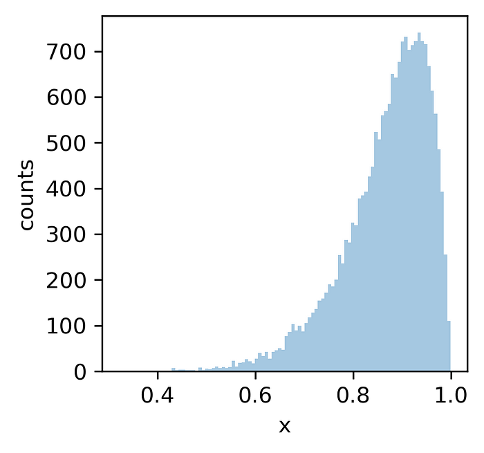
To get a sample from the Kumaraswamy distribution, we just need to generate a sample from the standard uniform distribution and feed it to the Kumaraswamy quantile function with the desired parameters (we will use a=10, b=2):

uni_sample = st.uniform.rvs(0, 1, 20000)
kumaraswamy_sample = kumaraswamy_q(uni_sample, 10, 2)

sample from the Kumaraswamy distribution (a=10, b=2) — image by author

Now we are ready to use the sample and estimate the parameters of the Kumaraswamy distribution:

kumaraswamy_mle(kumaraswamy_sample)
(10.076626243961558, 1.992270000094411)

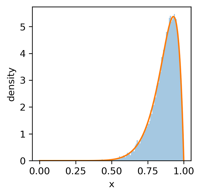
Kumaraswamy distribution (with parameters estimated using MLE) fitted to our sample — image by author

As you can see, the estimated parameters are very close to the true values we used while generating the sample. Easy, isn't it?

Although MLE is a very powerful tool, it has its limitations. For some distributions, it cannot estimate all parameters ( you need to know the true value of some parameters to make it work or just use a different estimation method), or its estimates are biased. That's why it's always good to do some background research on your distribution and make sure you can calculate the right thing.