Have you ever wondered how to measure the actual size of objects within an image? It is definitely possible to do so using OpenCV functionalities! In this article I would like to give a tutorial on that.

The main idea of the algorithm is actually quite straightforward. Look at the sample image we are going to work with in Figure 1 below.

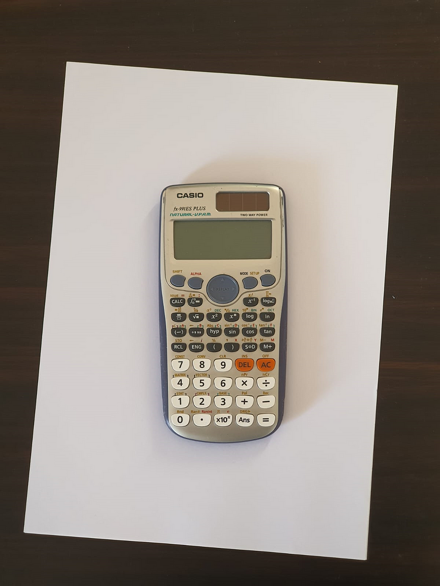Figure 1. A sample image used in this tutorial.

The objective of this tutorial is to estimate the width and height of the calculator in millimeters. In order to do so, we need an object which the size is already known as a reference length. This is essentially the reason that we employ the plain paper as the object background. The paper size is A4, meaning that it has the width and height of 210 mm and 297 mm, respectively. We can then obtain the estimated calculator size with the help of these numbers.

Before we begin, I want you to know that this article is divided into several chapters:

1. Importing Modules and Parameters Initialization
2. Image Loading and Preprocessing
3. Finding Paper Contour
4. Perspective Transformation
5. Finding Object Contours
6. Edge Length Calculation
7. Putting Everything in a Single Function

Now, let’s start from the first one.

1. Importing Modules and Parameters Initialization

Just like other Python projects, the very first thing I want to do is to import all the required modules. In this case, most of our work is going to be done using both cv2 and numpy, whereas matplotlib is merely used to display images.

# Codeblock 1
import cv2
import numpy as np
import matplotlib.pyplot as plt

As the modules have been imported, we are going to initialize some parameters that we need for future computations which you can see in Codeblock 2 below. The SCALE variable is essentially used because we don’t want our resulting image to be too small. Meanwhile, the PAPER_W and PAPER_H denote the paper width and height in millimters.

# Codeblock 2
SCALE = 3
PAPER_W = 210 * SCALE
PAPER_H = 297 * SCALE

And that’s it. This is the end of the first chapter as there is nothing more to say in this part.

2. Image Loading and Preprocessing

Afterwards, we are going to create a function named load_image() and show_image() which I think the name of the two functions are self-explanatory. The details of those can be seen in Codeblock 3. You can see below that I define the scale parameter (lowercase), in which my intention is to make the input image become a bit smaller since the original image resolution is very high. But well, technically speaking you can also make it even larger instead by passing a value greater than 1.

The show_image() function, on the other hand, implements cv2.cvtColor() that is employed to convert the color channel from BGR to RGB. Such a conversion is necessary because Matplotlib works differently from OpenCV in terms of color channel order.

# Codeblock 3
def load_image(path, scale=0.7):
    img = cv2.imread(path)
    img_resized = cv2.resize(img, (0,0), None, scale, scale)
    return img_resized

def show_image(img):
    img = cv2.cvtColor(img, cv2.COLOR_BGR2RGB)
    plt.figure(figsize=(6,8))
    plt.xticks([])
    plt.yticks([])
    plt.imshow(img)
    plt.show()

As the two functions above have been initialized, now that we can use it to actually load the image. Here I decided to leave the scale parameter to its default value (0.7) which causes the loaded image having the size of 1120×840 px (the original size is 1600×1200 px).

# Codeblock 4
img_original = load_image(path='images/1.jpeg')
show_image(img_original)
print(img_original.shape)

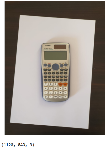Figure 2. The image to be processed has the dimension of 1120 x 840 px.

The image I displayed above is stored in img_original. The subsequent step to do is to preprocess this image using a sequence of image processing techniques, namely grayscale conversion (#1), blurring (#2), Canny edge detection (#3), dilation (#5) and closing (#6). All these steps are wrapped in the preprocess_image() function in Codeblock 5.

# Codeblock 5
def preprocess_image(img, thresh_1=57, thresh_2=232):
    img_gray  = cv2.cvtColor(img, cv2.COLOR_BGR2GRAY)      #1
    img_blur  = cv2.GaussianBlur(img_gray, (5,5), 1)       #2
    img_canny = cv2.Canny(img_blur, thresh_1, thresh_2)    #3

    kernel = np.ones((3,3))    #4
    img_dilated = cv2.dilate(img_canny, kernel, iterations=1)    #5
    img_closed = cv2.morphologyEx(img_dilated, cv2.MORPH_CLOSE,
                                  kernel, iterations=4)          #6

    img_preprocessed = img_closed.copy()

    img_each_step = {'img_dilated': img_dilated,
                     'img_canny'  : img_canny,
                     'img_blur'   : img_blur,
                     'img_gray'   : img_gray}

    return img_preprocessed, img_each_step

In the line marked by #2, the argument of (5,5) and 1 indicate Gaussian filter size and the Gaussian distribution standard deviation, respectively. Meanwhile, thresh_1 and thresh_2 in line #3 are the two thresholds used by Canny edge detector to capture weak and strong edges. In this case, I decided to set thresh_1 to 57 and thresh_2 to 232, in which these numbers were determined by trial and error. Next, we initialize a 3×3 kernel where all elements of the kernel are set to 1 (line marked by #4). This all-ones kernel will then be used in the dilation and closing process as the structuring element.

The preprocess_image() function returns two values: the completely preprocessed image (stored in img_preprocessed) and the result of each preprocessing stage (stored in img_each_step as a dictionary). The outputs of the function can be seen in Figure 3. The image to be brought to the next process is the img_preprocessed (the rightmost).

# Codeblock 6
img_preprocessed, img_each_step = preprocess_image(img_original)
show_image(img_each_step['img_gray'])
show_image(img_each_step['img_blur'])
show_image(img_each_step['img_canny'])
show_image(img_each_step['img_dilated'])
show_image(img_preprocessed)

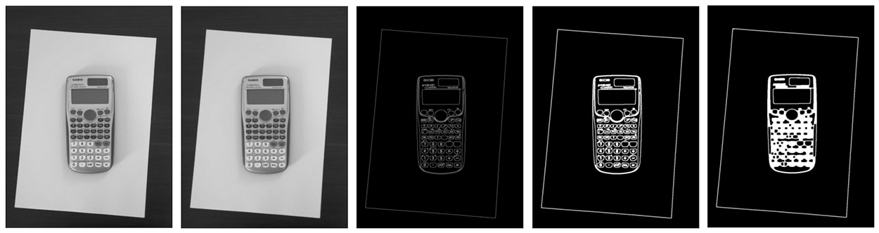Figure 3. The sequence of image transformations from left to right: grayscaling, blurring, edge detection, dilation, and closing.

3. Finding Paper Contour

The next thing to be done after obtaining the preprocessed image is to find the contours using the codes displayed in Codeblock 7. You can see there that we employ cv2.findContours() to do so (#1). We also pass cv2.RETR_EXTERNAL as the input argument for the mode parameter, in which it is used because we are only interested in capturing the outermost contours detected within the image, i.e., the paper. For now, the calculator object is just going to be ignored. The detected contours themselves will then be drawn using cv2.drawContours() (#2).

# Codeblock 7
def find_contours(img_preprocessed, img_original, epsilon_param=0.04):
    contours, hierarchy = cv2.findContours(image=img_preprocessed,
                                           mode=cv2.RETR_EXTERNAL,
                                           method=cv2.CHAIN_APPROX_NONE)  #1

    img_contour = img_original.copy()
    cv2.drawContours(img_contour, contours, -1, (203,192,255), 6)  #2

    polygons = []
    for contour in contours:
        epsilon = epsilon_param * cv2.arcLength(curve=contour,
                                                closed=True)  #3
        polygon = cv2.approxPolyDP(curve=contour,
                                   epsilon=epsilon, closed=True)  #4

        polygon = polygon.reshape(4, 2)  #5
        polygons.append(polygon)

        for point in polygon:
            img_contour = cv2.circle(img=img_contour, center=point,
                                     radius=8, color=(0,240,0),
                                     thickness=-1)  #6

    return polygons, img_contour

Not only that, here I also attempt to approximate the contour shape using cv2.approxPolyDP() (#4). The objective of this line of code is to obtain the four corners of the paper contour, in which the coordinates are then stored in polygon. One thing that we need to pay attention to is the epsilon parameter used in line #3. A small epsilon value tends to result in the detection of a larger number of corners, while on the other hand large epsilon causes the cv2.approxPolyDP() function to capture the general shape of the polygon, i.e., less corners. It is important to pay attention to the epsilon value since we need to ensure that the function will capture exactly four corner points.

Array reshaping needs to be performed (#5) because the original output of cv2.approxPolyDP() is in the format (number of corners, 1, 2), where the middle axis is irrelevant in our case. Hence, we can safely discard it. In addition to the find_contours() function, here we are also going to display the corners using cv2.circle() (#6). This function will then return the corner coordinates themselves (polygon) and the image with the highlighted contours (img_contour).

The Codeblock 8 below shows how I call the find_contours() function. Here I decided to set the epsilon_param to 0.04. You will probably need to change this value if you are using your own pictures, especially if the lighting characteristics is different from my image. The output of the below codeblock, which is displayed in Figure 4, shows what the contours and corners look like. I do also print the coordinates stored in polygon[0]. In case you’re wondering, the indexer of 0 is used because essentially the find_contours() function is capable of capturing multiple contours, while in this case the only external contour that we have is the paper itself. In addition to that, it might be worth noting that the coordinates stored in polygons are in (x,y) format, not (y,x).

# Codeblock 8
polygons, img_contours = find_contours(img_preprocessed,
                                       img_original,
                                       epsilon_param=0.04)
show_image(img_contours)
polygons[0]

Figure 4. What the contours (pink) and corners (green) look like.

4. Perspective Transformation

As the paper corner coordinates have been detected, now that we are going to warp the image according to those four points. The objective of this process is to straighten the paper before we start finding the object contours.

Reordering Coordinates

When it comes to the straightening process, one thing that we need to know is that the detected polygon corners may not be ordered thanks to the nature of the cv2.approxPolyDP() function. To make all these four points ordered, we need to create a function specialized to do it. The function that I am talking about is called reorder_coords() which the details can be seen in Codeblock 9.

# Codeblock 9
def reorder_coords(polygon):
    rect_coords = np.zeros((4, 2))

    add = polygon.sum(axis=1)
    rect_coords[0] = polygon[np.argmin(add)]    # Top left
    rect_coords[3] = polygon[np.argmax(add)]    # Bottom right

    subtract = np.diff(polygon, axis=1)
    rect_coords[1] = polygon[np.argmin(subtract)]    # Top right
    rect_coords[2] = polygon[np.argmax(subtract)]    # Bottom left

    return rect_coords

The above function works by taking both the argmin and argmax from the addition and subtraction of the two coordinate numbers. These lines of codes magically put the top-left, top-right, bottom-left, and bottom-right corners at index 0, 1, 2 and 3, respectively. We can then apply this function to the points stored in polygon[0] as shown in Codeblock 10.

# Codeblock 10
rect_coords = np.float32(reorder_coords(polygons[0]))
rect_coords

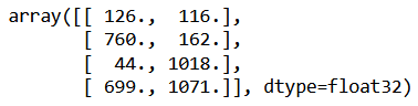Figure 5. The four corner points of the paper that we have ordered using reorder_coords() function.

Later on, the reordered paper corner coordinates above (rect_coords) are going to act as the source of the transformation, while the transformation destination (paper_coords) is determined by the actual paper size, i.e., PAPER_W and PAPER_H. Look at Codeblock 11 to see how I manually arrange the points stored for paper_coords. One thing to keep in mind here is that the order of destination coordinates needs to exactly match with the order of the source coordinates, which is the reason that we implemented the reorder_coords() function for reordering our source coordinates.

# Codeblock 11
paper_coords = np.float32([[0,0],                # Top left
                           [PAPER_W,0],          # Top right
                           [0,PAPER_H],          # Bottom left
                           [PAPER_W,PAPER_H]])   # Bottom right
paper_coords

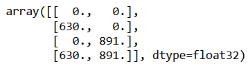Figure 6. The destination coordinates used for image transformation.

In addition to the Codeblock 10 and 11, you might probably notice that I converted the array datatype to float32. In fact, I tried to use other datatypes such as int32 and float64 and turns out both of those caused the cv2.getPerspectiveTransform() function in the subsequent codeblock to return an error.

Creating Transformation Matrix

At this point, we have already got rect_coords and paper_coords. We are now ready to use them to warp the original image using cv2.getPerspectiveTransform() and cv2.warpPerspective() as you can see in Codeblock 12 below. In order to make the code cleaner, I put them inside another function named warp_image().

# Codeblock 12
def warp_image(rect_coords, paper_coords, img_original, pad=5):

    matrix = cv2.getPerspectiveTransform(src=rect_coords,
                                         dst=paper_coords)   #1
    img_warped = cv2.warpPerspective(img_original, matrix,
                                      (PAPER_W, PAPER_H))    #2

    warped_h = img_warped.shape[0]
    warped_w = img_warped.shape[1]
    img_warped = img_warped[pad:warped_h-pad, pad:warped_w-pad]  #3

    return img_warped

Let’s dive into the above function. We first employ the cv2.getPerspectiveTransform() (#1) to create the so-called transformation matrix. The transformation matrix itself, which has the dimension of 3 × 3, stores an information regarding how an image can be transformed from one perspective to another. The matrix will then actually be used to transform the original image using cv2.warpPerspective() (#2). We then store the transformed image in a variable named img_warped. In addition to the warp_image() function, we are going to discard the area near the image border (#3) since the resulting image may contain a narrow unwanted black region at the edges.

The use of warp_image() function is demonstrated in Codeblock 13 in which the output is displayed in Figure 7.

# Codeblock 13
img_warped = warp_image(rect_coords, paper_coords, img_original)
show_image(img_warped)
print(img_warped.shape)

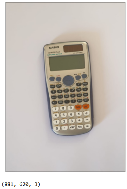Figure 7. The warped image.

5. Finding Object Contours

As the original image has been warped according to the paper shape, next I will do the exact same process in order to detect the calculator object, i.e., image preprocessing and contour searching. Since the processes to be done are the same to the previous ones, hence we can simply reuse the functions we defined earlier. In this case, our inner contours, i.e., calculator buttons, will be ignored thanks to the use of cv2.RETR_EXTERNAL that we implemented back in Codeblock 7.

Now the Codeblock 14 and 15 show how preprocessing and contour finding is done.

# Codeblock 14
img_warped_preprocessed, _ = preprocess_image(img_warped)
show_image(img_warped_preprocessed)

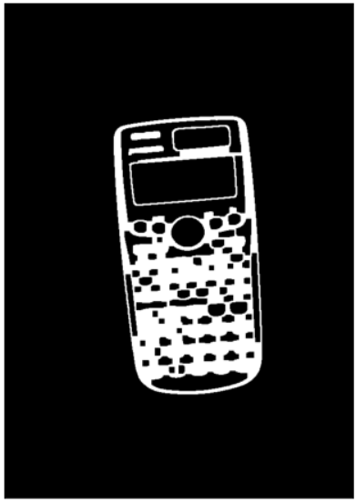Figure 8. The warped image that has been preprocessed.

# Codeblock 15
polygons_warped, img_contours_warped = find_contours(img_warped_preprocessed,
                                                     img_warped,
                                                     epsilon_param=0.04)
show_image(img_contours_warped)
polygons_warped[0]

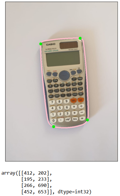Figure 9. The detected contour (pink) and corners (green).

As the codes in the two Codeblocks above have been run, now that all corner coordinates (green circles) are stored in polygons_warped. These four coordinate values are actually the ones to be utilized to estimate edge lengths.

6. Edge Lengths Calculation

In this case we assume that all objects on top of the paper are rectangle. Thus, object’s height can be estimated by calculating the Euclidean distance between its top-left corner and its bottom-left corner (Codeblock 16 #2). Meanwhile, the width can be obtained by calculating the same distance metric between object’s top-left corner and its top-right corner (#3). Furthermore, we need to remember that the detected corners returned by find_contours() are still unordered. Hence, we need to call reorder_coords() beforehand (#1). The last thing I want to emphasize in Codeblock 16 is that the estimated height and width are now stored in an array named sizes in that respective order (#4)

# Codeblock 16
def  calculate_sizes(polygons_warped):

rect_coords_list = []
for polygon in polygons_warped:
rect_coords = np.float32(reorder_coords(polygon)) #1
rect_coords_list.append(rect_coords)

heights = []
widths = []
for rect_coords in rect_coords_list:
height = cv2.norm(rect_coords[0], rect_coords[2], cv2.NORM_L2) #2
width = cv2.norm(rect_coords[0], rect_coords[1], cv2.NORM_L2) #3

heights.append(height)
widths.append(width)

heights = np.array(heights).reshape(-1,1)
widths = np.array(widths).reshape(-1,1)

sizes = np.hstack((heights, widths)) #4

return sizes, rect_coords_list

sizes, rect_coords_list = calculate_sizes(polygons_warped)
sizes

Figure 10. The calculator height (index 0) and width (index 1) in pixels.

Convert to Millimeters

However, we need to keep in mind that the output in Figure 10 is still in the number of pixels. To convert these values to millimeters, we need to create a separate function for that, which I name convert_to_mm() (Codeblock 17). This function works by taking the ratio of paper length in millimeters and in pixels (#1 and #2). Then, we can obtain the actual millimeters length by multiplying the ratio value (scale_h and scale_w) with the calculator size that is still in pixels (#3 and #4).

# Codeblock 17
def convert_to_mm(sizes_pixel, img_warped):
    warped_h = img_warped.shape[0]
    warped_w = img_warped.shape[1]

    scale_h = PAPER_H / warped_h    #1
    scale_w = PAPER_W / warped_w    #2

    sizes_mm = []

    for size_pixel_h, size_pixel_w in sizes_pixel:
        size_mm_h = size_pixel_h * scale_h / SCALE    #3
        size_mm_w = size_pixel_w * scale_w / SCALE    #4

        sizes_mm.append([size_mm_h, size_mm_w])

    return np.array(sizes_mm)

sizes_mm = convert_to_mm(sizes, img_warped)
sizes_mm

Figure 11. The calculator height and width that have been converted to millimeters.

Up until this point, we have successfully obtained the length of the edges in millimeters. Now that we are going to display these values in form of a text written on the warped image. The entire processes done for this are put inside the write_size() function. After the function has been initialzed, we can directly call it as shown in line #1 in Codeblock 18. The output of this code can be seen in Figure 12.

And well, it seems like our codes work as expected.

# Codeblock 18
def write_size(rect_coords_list, sizes, img_warped):

    img_result = img_warped.copy()

    for rect_coord, size in zip(rect_coords_list, sizes):

        top_left = rect_coord[0].astype(int)
        top_right = rect_coord[1].astype(int)
        bottom_left = rect_coord[2].astype(int)

        cv2.line(img_result, top_left, top_right, (255,100,50), 4)
        cv2.line(img_result, top_left, bottom_left, (100,50,255), 4)

        cv2.putText(img_result, f'{np.int32(size[0])} mm',
                    (bottom_left[0]-20, bottom_left[1]+50),
                    cv2.FONT_HERSHEY_DUPLEX, 1, (100,50,255), 1)

        cv2.putText(img_result, f'{np.int32(size[1])} mm',
                    (top_right[0]+20, top_right[1]+20),
                    cv2.FONT_HERSHEY_DUPLEX, 1, (255,100,50), 1)

    return img_result

img_result = write_size(rect_coords_list, sizes_mm, img_warped)  #1
show_image(img_result)
print(img_result.shape)

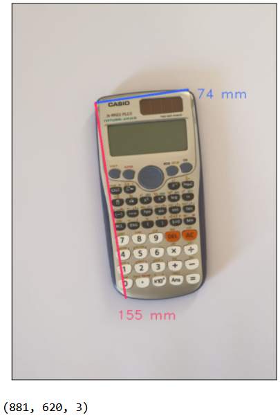Figure 12. Putting texts on the image.

7. Putting Everything in a Single Function

All the steps we did above seem pretty long since I try to explain every part of the code use din this project. In fact, all the codes you see so far can be wrapped in a single function which I name measure_size() in Codeblock 19. Using this function, we can simply pass the image to be processed alongside the parameters to do all the works we just done.

# Codeblock 19
def measure_size(path, img_original_scale=0.7,
                 PAPER_W=210, PAPER_H=297, SCALE=3,
                 paper_eps_param=0.04, objects_eps_param=0.05,
                 canny_thresh_1=57, canny_thresh_2=232):

    PAPER_W = PAPER_W * SCALE
    PAPER_H = PAPER_H * SCALE

    # Loading and preprocessing original image.
    img_original = load_image(path=path, scale=img_original_scale)
    img_preprocessed, img_each_step = preprocess_image(img_original,
                                                       thresh_1=canny_thresh_1,
                                                       thresh_2=canny_thresh_2)

    # Finding paper contours and corners.
    polygons, img_contours = find_contours(img_preprocessed,
                                           img_original,
                                           epsilon_param=paper_eps_param)

    # Reordering paper corners.
    rect_coords = np.float32(reorder_coords(polygons[0]))

    # Warping image according to paper contours.
    paper_coords = np.float32([[0,0],
                               [PAPER_W,0],
                               [0,PAPER_H],
                               [PAPER_W,PAPER_H]])
    img_warped = warp_image(rect_coords, paper_coords, img_original)

    # Preprocessing the warped image.
    img_warped_preprocessed, _ = preprocess_image(img_warped)

    # Finding contour in the warped image.
    polygons_warped, img_contours_warped = find_contours(img_warped_preprocessed,
                                                         img_warped,
                                                         epsilon_param=objects_eps_param)

    # Edge langth calculation.
    sizes, rect_coords_list = calculate_sizes(polygons_warped)
    sizes_mm = convert_to_mm(sizes, img_warped)
    img_result = write_size(rect_coords_list, sizes_mm, img_warped)

    return img_result

Once the measure_size() function has been created, now that we can test it on several test cases. And well, the outputs shown in Figure 13 show that our approach on estimating object size works pretty well for different rectangular-shaped objects.

# Codeblock 20
show_image(measure_size('images/1.jpeg'))
show_image(measure_size('images/2.jpeg'))
show_image(measure_size('images/3.jpeg'))
show_image(measure_size('images/4.jpeg'))
show_image(measure_size('images/5.jpeg'))
show_image(measure_size('images/6.jpeg', objects_eps_param=0.1))

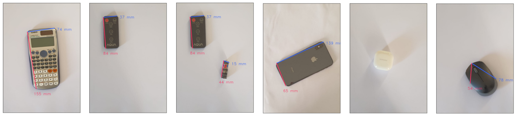Figure 13. Results on other images.

Limitations

Even though in many cases our approach is working properly, yet this does not necessarily mean that our work is perfect, even in a controlled environment. If you take a look a bit closely, you might notice that most of the predicted corners are not really located at the actual corner location, which might cause a bit of imprecision in the measurement. This is essentially because the corner points determination highly relies on the quality of the binary image, i.e., image after closing operation. Such a thing implies that input parameter value determination is very crucial in this case.

Furthermore, if we take a look at the second image from the right in Figure 13, you can see that the object dimension is not getting printed. This is probably because the contours are not detected quite well thanks to the subtle color difference between the object and the paper. Also, in our last test image (the rightmost one), it appears that our implementation struggles to accurately measure the size of an object with curved corners, despite its overall rectangular appearance.

That’s pretty much for today’s article. Hope you learn something new from here. Thanks for reading!

Note: the codes and other resources used in this writing are available in my GitHub repository.

If you enjoyed this article and want to learn about OpenCV and image processing, check out my comprehensive course on Udemy: Image Processing with OpenCV. You’ll gain hands-on experience and master essential techniques.