Bootstrapping Explained Simply: Resampling for Better Predictions

Imagine you wake up one morning and someone hands you a single slice of pizza from a party you weren’t invited to. They ask: “Based on this one slice, what was the entire party like?”

You could shrug and say, “I don’t know — I only have one slice.” Or you could do something cleverer: taste it, study its crust, weigh its toppings, and use everything you know about this one slice to make intelligent guesses about all the slices you never got to try.

That, in essence, is bootstrapping — one of the most quietly powerful ideas in modern statistics and machine learning. No fancy equations needed to understand it. No PhD required. Just a willingness to trust that the data you have can tell you a surprising amount about the data you don’t.

The Pizza Party Analogy: What Is Bootstrapping, Really?

Let’s say you want to know the average slice weight at a pizza party of 500 guests. But you can only grab 10 slices before the host kicks you out.

You weigh your 10 slices. You get an average. But how confident are you in that average? What if you’d grabbed a different 10 slices — would the average be wildly different?

This is the fundamental problem in statistics: we always work with samples, but we want to say something about the whole population.

Traditional statistics had one answer: math. Derive formulas. Make assumptions about the shape of your data (it’s normally distributed, they’d say). Hope for the best.

Then in 1979, a Stanford statistician named Bradley Efron had a different idea.

“The bootstrap is a computer-based method for statistical inference that can be used for a wide variety of problems.”* — Bradley Efron, creator of the Bootstrap me*thod

His idea? Instead of relying on assumptions, pretend your sample is the whole world — and resample from it.

Here’s how that works with your pizza slices:

• You have 10 slices. Write each weight on a card.
• Put all 10 cards in a hat.
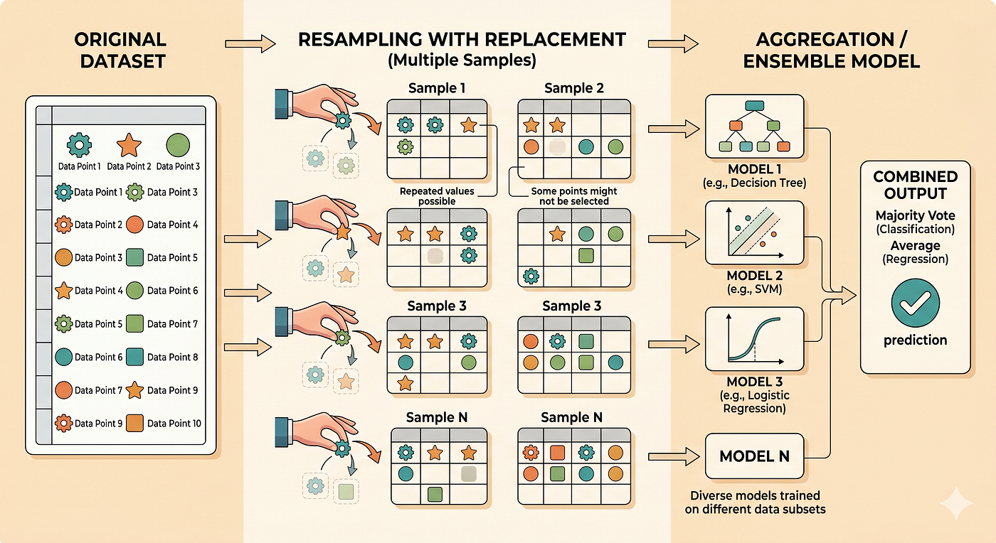
• Draw a card, write it down, put it back. Repeat 10 times. You now have a new “fake” sample of 10 slices — some weights may repeat, some may not appear at all.
• Calculate the average of this new sample.
• Put all 10 cards back in the hat. Repeat the whole process 1,000 times.
• Now you have 1,000 averages. Look at how they’re spread out. That spread tells you how uncertain your original estimate was.

That’s bootstrapping. You simulate the variability of the world by resampling from the world you already observed.

The word itself comes from the phrase “pulling oneself up by one’s own bootstraps” — doing something seemingly impossible using only what you already have.

Why “With Replacement” Matters

The single most important detail: you always draw with replacement.

Think of it like shuffling a deck, drawing a card, noting it, and then putting it back before drawing again. This means:

• The same data point can appear multiple times in a bootstrap sample.
• Some data points may not appear at all.
• Each bootstrap sample is a slightly different version of your original data.

This is by design. It simulates the randomness of the world. If you drew without replacement, every bootstrap sample would be identical to the original — useless.

On average, each bootstrap sample contains about 63.2% of the original unique data points. The rest are duplicates. This quirky number comes from probability theory: as sample size grows, the fraction of unique items selected approaches 1–1/e ≈ 0.632.

What Can You Estimate with Bootstrapping?

Pretty much anything you can calculate from a dataset:

What You Want to Know What Bootstrap Gives You Mean / Median Confidence interval around your estimate Standard deviation How stable is your spread? Correlation between variables Is this relationship real or noise? Model accuracy How will this model generalize? A/B test difference Is the effect real or just luck?

The bootstrap confidence interval is particularly powerful. Instead of using a formula that assumes normality, you just look at the 2.5th and 97.5th percentile of your 1,000 bootstrap estimates — that’s your 95% confidence interval. No assumptions needed.

“The great thing about the bootstrap is that it doesn’t require you to know the distribution of the statistic you’re interested in.”* — Trevor Hastie, co-author* of The Elements of Statistical Learning

Bootstrapping in Machine Learning

Here’s where things get exciting. The same idea that helps statisticians understand uncertainty becomes, in machine learning, a tool for building better models.

1. Bagging (Bootstrap Aggregating)

In 1994, Leo Breiman took Efron’s idea and asked: What if we trained not one model, but many models — each on a different bootstrap sample of the data?

The result was Bagging (Bootstrap Aggregating), and it changed machine learning forever.

Here’s the intuition:

• One decision tree trained on your data might overfit — it memorizes noise.
• Train 100 decision trees, each on a slightly different bootstrap sample of the same data. Each tree will be a little different — different splits, different patterns emphasized.
• When predicting, average their outputs (for regression) or take a majority vote (for classification).

The result is dramatically more stable and accurate than any single tree.

“Bagging can push a good but unstable procedure a significant step towards optimality.”* — Leo Breiman, inventor of Bagging and Random For*ests

2. Random Forests

Breiman went even further in 2001. He took bagging and added one more twist: at each split in each tree, only a random subset of features is considered. This creates even more diversity among the trees.

The result? Random Forests — one of the most reliable and widely used algorithms in all of machine learning.

Every Random Forest is, at its heart, a bootstrap idea: use the data you have, resample it creatively, and combine many imperfect views into one robust truth.

3. Gradient Boosting and Beyond

While gradient boosting (XGBoost, LightGBM) doesn’t use bootstrapping in the same way, the spirit is similar: build models sequentially, each correcting the errors of the last. The diversity of perspectives is still central.

4. Model Evaluation: Out-of-Bag Error

Here’s a beautiful bonus of bootstrap sampling in machine learning. Remember how each bootstrap sample leaves out ~36.8% of the data? Those left-out data points are called the Out-of-Bag (OOB) sample.

Since those points weren’t used to train that particular tree, you can use them to evaluate it — for free, without needing a separate validation set.

Random Forests use OOB error as a built-in, honest estimate of model performance.

Let’s Code It: Bootstrap in Python from Scratch

Enough theory. Let’s see bootstrapping in action with clean, beginner-friendly Python code.

Part 1: Building a Bootstrap Confidence Interval

import numpy as np
import matplotlib.pyplot as plt

# --- Our "sample" data ---
# Imagine these are the weights (in grams) of 20 pizza slices we measured.
np.random.seed(42)
pizza_weights = np.array([
    180, 195, 210, 175, 220, 190, 185, 205, 215, 178,
    200, 188, 225, 170, 198, 212, 183, 207, 193, 201
])

# Our observed mean
observed_mean = np.mean(pizza_weights)
print(f"Observed Mean: {observed_mean:.2f}g")

# --- Bootstrap ---
n_bootstraps = 10_000
bootstrap_means = []

for _ in range(n_bootstraps):
    # Resample WITH replacement
    bootstrap_sample = np.random.choice(pizza_weights, size=len(pizza_weights), replace=True)
    bootstrap_means.append(np.mean(bootstrap_sample))

bootstrap_means = np.array(bootstrap_means)

# --- Confidence Interval ---
lower = np.percentile(bootstrap_means, 2.5)
upper = np.percentile(bootstrap_means, 97.5)

print(f"\n95% Bootstrap Confidence Interval:")
print(f"  Lower bound: {lower:.2f}g")
print(f"  Upper bound: {upper:.2f}g")
print(f"\nInterpretation: We're 95% confident the true average")
print(f"pizza weight is between {lower:.1f}g and {upper:.1f}g")

# --- Visualise the distribution ---
plt.figure(figsize=(10, 5))
plt.hist(bootstrap_means, bins=60, color='tomato', edgecolor='white', alpha=0.85)
plt.axvline(observed_mean, color='black', linestyle='--', linewidth=2, label=f'Observed Mean: {observed_mean:.1f}g')
plt.axvline(lower, color='navy', linestyle=':', linewidth=2, label=f'95% CI Lower: {lower:.1f}g')
plt.axvline(upper, color='navy', linestyle=':', linewidth=2, label=f'95% CI Upper: {upper:.1f}g')
plt.title('Bootstrap Distribution of Sample Means', fontsize=15)
plt.xlabel('Bootstrap Sample Mean (grams)', fontsize=12)
plt.ylabel('Frequency', fontsize=12)
plt.legend()
plt.tight_layout()
plt.savefig('bootstrap_distribution.png', dpi=150)
plt.show()

What’s happening here?

• We have 20 pizza slice weights (our sample).
• We draw 10,000 bootstrap samples, each of size 20, with replacement.
• We compute the mean of each bootstrap sample.
• We look at the 2.5th and 97.5th percentiles of those 10,000 means — that’s our confidence interval.

No formula. No assumption of normality. Just resampling.

Part 2: Bagging a Decision Tree from Scratch

from sklearn.datasets import load_breast_cancer
from sklearn.tree import DecisionTreeClassifier
from sklearn.model_selection import train_test_split
from sklearn.metrics import accuracy_score
import numpy as np

# --- Load Dataset ---
data = load_breast_cancer()
X, y = data.data, data.target

X_train, X_test, y_train, y_test = train_test_split(
    X, y, test_size=0.2, random_state=42
)

n_samples = X_train.shape[0]
n_bootstraps = 100

# --- Manual Bagging ---
predictions = []

for i in range(n_bootstraps):
    # Step 1: Create a bootstrap sample
    indices = np.random.choice(n_samples, size=n_samples, replace=True)
    X_boot = X_train[indices]
    y_boot = y_train[indices]

    # Step 2: Train a Decision Tree on this bootstrap sample
    tree = DecisionTreeClassifier(max_depth=5, random_state=i)
    tree.fit(X_boot, y_boot)

    # Step 3: Predict on the test set
    pred = tree.predict(X_test)
    predictions.append(pred)

# --- Aggregate: Majority Vote ---
predictions = np.array(predictions)  # Shape: (100, n_test_samples)
majority_vote = np.apply_along_axis(
    lambda x: np.bincount(x).argmax(),
    axis=0,
    arr=predictions
)

bagging_accuracy = accuracy_score(y_test, majority_vote)

# --- Compare: Single Decision Tree ---
single_tree = DecisionTreeClassifier(max_depth=5, random_state=42)
single_tree.fit(X_train, y_train)
single_accuracy = accuracy_score(y_test, single_tree.predict(X_test))

print("=" * 45)
print(f"  Single Decision Tree Accuracy:  {single_accuracy:.4f}")
print(f"  Bagged Trees Accuracy (100):    {bagging_accuracy:.4f}")
print(f"  Improvement:                   +{(bagging_accuracy - single_accuracy):.4f}")
print("=" * 45)

Expected Output (approximate):

=============================================
  Single Decision Tree Accuracy:  0.9298
  Bagged Trees Accuracy (100):    0.9561
  Improvement:                   +0.0263
=============================================

Notice the improvement. You didn’t add more data, you didn’t build a fancier model — you just resampled cleverly.

Part 3: Out-of-Bag (OOB) Evaluation

from sklearn.ensemble import RandomForestClassifier

# Random Forest with OOB scoring enabled
rf = RandomForestClassifier(
    n_estimators=200,
    oob_score=True,       # <-- This is the magic switch
    random_state=42,
    n_jobs=-1
)
rf.fit(X_train, y_train)

test_accuracy = accuracy_score(y_test, rf.predict(X_test))

print(f"OOB Score (free validation):  {rf.oob_score_:.4f}")
print(f"Test Set Accuracy:            {test_accuracy:.4f}")
print(f"\nOOB score is a reliable estimate of test performance")
print(f"computed entirely from bootstrap leftovers — no extra data needed!")

The OOB score is often surprisingly close to the actual test accuracy. That’s not magic — it’s just clever use of what bootstrapping naturally gives you for free.

Limitations of Bootstrapping

Bootstrapping is powerful, but it’s not a miracle. Here’s where it can stumble:

1. Small Samples If your original dataset has only 5 or 10 data points, resampling from them can’t create much new information. The bootstrap works best when the sample is a reasonable representation of the population.

2. Extreme Values and Heavy Tails If your data has rare extreme outliers, the bootstrap may over or underestimate their frequency. When rare events dominate your statistic of interest, be cautious.

3. Time Series Data With sequential data, observations aren’t independent — today’s stock price depends on yesterday’s. Standard bootstrapping breaks this dependence. Special methods like the block bootstrap are needed.

4. Computational Cost Running 10,000 bootstrap samples of a complex model can be slow. It’s tractable for many use cases, but not always free.

“Like all statistical methods, the bootstrap has its weaknesses. Understanding when not to use a method is just as important as knowing when to use it.”* — Robert Tibshirani, co-author* of The Elements of Statistical Learning

Key Takeaways (The Short Version)

• Bootstrap = Resample with replacement from your existing data, repeatedly, to simulate variability.
• It lets you estimate confidence intervals without mathematical assumptions about your data’s distribution.
• In ML, Bagging uses bootstrap samples to train many models and combine them — reducing variance and improving accuracy.
• Random Forests are the most famous descendant of this idea.
• Out-of-Bag evaluation gives you a free, honest model performance estimate using the data each tree never saw.
• It has limits: small data, time series, and computational cost all deserve attention.

Conclusion: The Audacity to Learn from What You Have

There’s something deeply human about bootstrapping. It’s the statistical equivalent of making do — of refusing to say “I don’t have enough” and instead asking “What can I learn from what I do have?”

Every time a Random Forest makes a prediction that saves a cancer diagnosis, or catches a fraudulent transaction, or recommends the song that makes your evening — somewhere underneath all that complexity is Efron’s 1979 insight: take what you have, resample it creatively, and listen to what the variation tells you.

Beginner or expert, that’s a lesson worth bootstrapping into everything you do.

References & Further Reading

• Efron, B. (1979). Bootstrap Methods: Another Look at the Jackknife. The Annals of Statistics.
• Breiman, L. (1996). Bagging Predictors. Machine Learning.
• Hastie, T., Tibshirani, R., & Friedman, J. The Elements of Statistical Learning (2nd ed.).
• Scikit-learn documentation: Ensemble Methods