BigMart Sales Prediction Project

This post is the day 2 post of my '10 days of machine learning projects' tutorial series. If you are new to my blog then you can check out Day 1 post here.

Without wasting any time let's dive into our today's tutorial.

Photo by Jon Cellier on Unsplash

DataSet

Download the dataset from here : https://www.kaggle.com/brijbhushannanda1979/bigmart-sales-data

Hypotheses Generation

It is always a good idea to generate some hypotheses before proceeding to any data science project.

We can separate this process into four levels: Product level, Store level, Customer level, and Macro level.

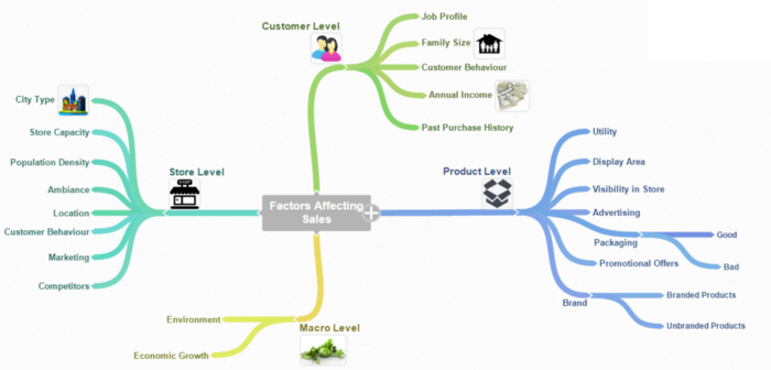
Source: Analytics Vidhya

Product level hypotheses:

1. Brand: Branded products have more trust of the customers so they should have high sales.
2. Visibility in Store: The location of the product placement also depends on the sales.
3. Display Area: Products that are placed at an attention-catching place should have more sales.
4. Utility: Daily use products have a higher tendency to sell compared to other products.
5. Packaging: Quality packaging can attract customers and sell more.

Store Level Hypotheses:

1. City type: Stores located in urban cities should have higher sales.
2. Store Capacity: One-stop shops are big in size so their sell should be high.
3. Population density: Densely populated areas have high demands so the store located in these areas should have higher sales.
4. Marketing: Stores having a good marketing division can attract customers through the right offers.

You can generate more hypotheses, these are some hypotheses that I think should be.

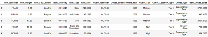
Take a look at the Data Structure

import pandas as pd
import numpy as np
import matplotlib.pyplot as plt
import seaborn as sns
%matplotlib inline
import warnings # Ignores any warning
warnings.filterwarnings("ignore")

train = pd.read_csv("/content/bigmart-sales-data/Train.csv")
test = pd.read_csv("/content/bigmart-sales-data/Test.csv")

train.head()

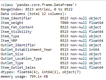
train.info()

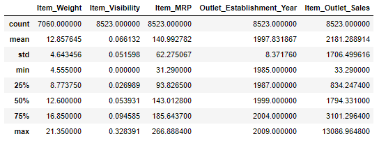
train.describe()

Overview of what we are going to cover:

1. Exploratory data analysis (EDA)
2. Data Pre-processing
3. Feature engineering
4. Feature Transformation
5. Modeling
6. Hyperparameter tuning

BigMart Sales Prediction

Exploratory data analysis (EDA)

We have made our hypotheses and now we are ready to do some data exploration and come up with some inference.

The goal for the EDA is to get some insight and if any irregularities are found we will correct that in the next section, Data Pre-Processing.

# Check for duplicates
idsTotal = train.shape[0]
idsDupli = train[train['Item_Identifier'].duplicated()]
print(f'There are {len(idsDupli)} duplicate IDs for {idsTotal} total entries')

Output:

There are 6964 duplicate IDs for 8523 total entries

This shows that our Item_Identifier has some duplicate values. since a product can exist in more than one store it is expected for this repetition.

1.1. Univariate Analysis

In Univariate analysis we will explore each variable in a dataset.

1.1.1. Distribution of the target variable: Item_Outlet_Sales

plt.figure(figsize=(12,7))
sns.distplot(train.Item_Outlet_Sales, bins = 25)
plt.xlabel("Item_Outlet_Sales")
plt.ylabel("Number of Sales")
plt.title("Item_Outlet_Sales Distribution")

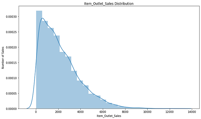
print ("Skew is:", train.Item_Outlet_Sales.skew())
print("Kurtosis: %f" % train.Item_Outlet_Sales.kurt())

Output:

Skew is: 1.1775306028542798
Kurtosis: 1.615877

We can see that our target variable is skewed towards the right. Therefore, we have to normalize it.

1.1.2. Numerical Predictors

Now we will consider our dependent variables. First of all, we will check for the numerical variables in our dataset:

num_features = train.select_dtypes(include=[np.number])
num_features.dtypes

Output:

Item_Weight                  float64
Item_Visibility              float64
Item_MRP                     float64
Outlet_Establishment_Year      int64
Item_Outlet_Sales            float64
dtype: object

We can see that out of 12 we have only 5 numeric variables.

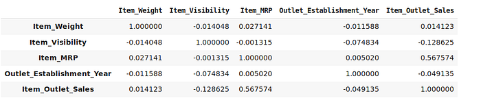
1.1.2.1. Correlation between Numerical Predictors and Target variable

Now let's check the correlation between our dependent variables and target variable:

corr=num_features.corr()
corr

corr['Item_Outlet_Sales'].sort_values(ascending=False)

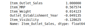
From the above result, we can see that Item_MRP have the most positive correlation and the Item_Visibility have the lowest correlation with our target variable. It is totally different from our initial hypotheses, this variables was expected to have high impact in the sales increase. Nevertheless, since this is not an expected behaviour and we should investigate.

1.1.3. Categorical Predictors

Now lets do some analysis on categorical variable and look at the variables that contain some insight on the hypotheses that we previously made.

1.1.3.1. Distribution of the variable Item_Fat_Content

sns.countplot(train.Item_Fat_Content)

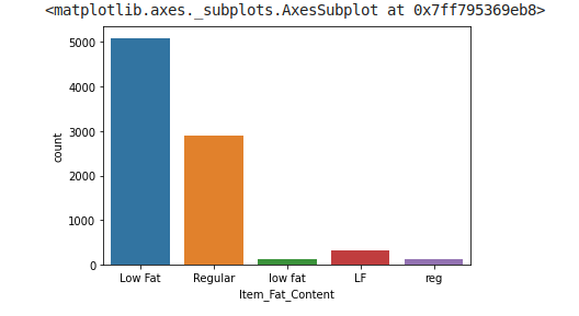
For Item_Fat_Content there are two possible type “Low Fat” or “Regular”. However, in our data it is written in different manner. We will Correct this.

1.1.3.2. Distribution of the variable Item_Type

sns.countplot(train.Item_Type)
plt.xticks(rotation=90)

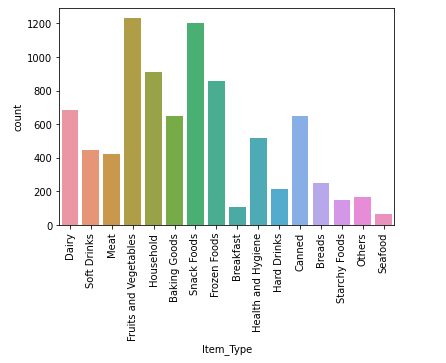
forItem_Type we have 16 different types of unique values and it is high number for categorical variable. Therefore we must try to reduce it.

1.1.3.3. Distribution of the variable Outlet_Size

sns.countplot(train.Outlet_Size)

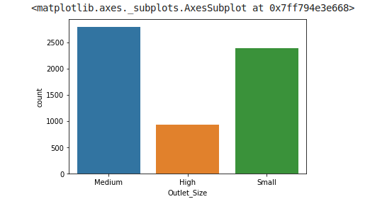
There seems to be less number of stores with size equals to “High”. It will be very interesting to see how this variable relates to our target.

1.1.3.4. Distribution of the variable Outlet_Location_Type

sns.countplot(train.Outlet_Location_Type)

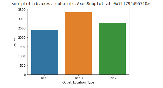
From the above graph we can see that Bigmart is a brand of medium and small size city compare to densely populated area.

1.1.3.5. Distribution of the variable Outlet_Type

sns.countplot(train.Outlet_Type)
plt.xticks(rotation=90)

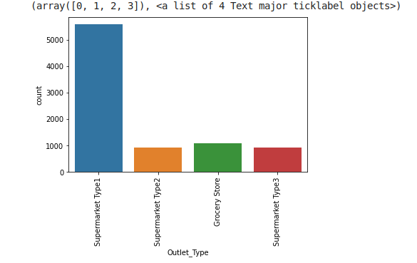
There seems like Supermarket Type2 , Grocery Store and Supermarket Type3 all have low numbers of stores, we can create a single category with all of three, but before doing this we must see their impact on target variable.

1.2. Bivariate Analysis

Now it time to see the relationship between our target variable and predictors.

1.2.1. Numerical Variables

1.2.1.1. Item_Weight and Item_Outlet_Sales analysis

plt.figure(figsize=(12,7))
plt.xlabel("Item_Weight")
plt.ylabel("Item_Outlet_Sales")
plt.title("Item_Weight and Item_Outlet_Sales Analysis")
plt.plot(train.Item_Weight, train["Item_Outlet_Sales"],'.', alpha = 0.3)

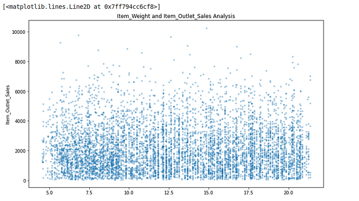
We saw previously that Item_Weight had a low correlation with our target variable. This plot shows there relation.

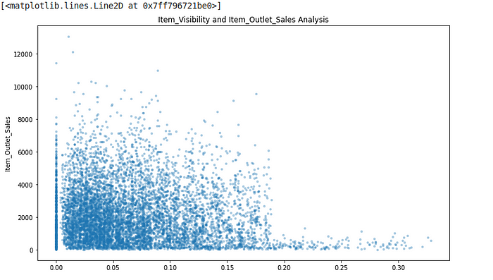
1.2.1.2. Item_Visibility and Item_Outlet_Sales analysis

plt.figure(figsize=(12,7))
plt.xlabel("Item_Visibility")
plt.ylabel("Item_Outlet_Sales")
plt.title("Item_Visibility and Item_Outlet_Sales Analysis")
plt.plot(train.Item_Visibility, train["Item_Outlet_Sales"],'.', alpha = 0.3)

1.2.1.3. Outlet_Establishment_Year and Item_Outlet_Sales analysis

Outlet_Establishment_Year_pivot = train.pivot_table(index='Outlet_Establishment_Year', 	values="Item_Outlet_Sales", aggfunc=np.median)
Outlet_Establishment_Year_pivot.plot(kind='bar', color='blue',figsize=(12,7))

plt.xlabel("Outlet_Establishment_Year")
plt.ylabel("Sqrt Item_Outlet_Sales")
plt.title("Impact of Outlet_Establishment_Year on Item_Outlet_Sales")
plt.xticks(rotation=0)
plt.show()

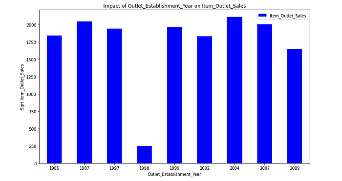
There seems to be no appreciable meaning between the year of store establishment and the sales for the items.

3.2.2. Categorical Variables

1.2.2.1. Impact of Item_Fat_Content onItem_Outlet_Sales

Item_Fat_Content_pivot = train.pivot_table(index='Item_Fat_Content', values="Item_Outlet_Sales", aggfunc=np.median)
Item_Fat_Content_pivot.plot(kind='bar', color='blue',figsize=(12,7))

plt.xlabel("Item_Fat_Content")
plt.ylabel("Item_Outlet_Sales")
plt.title("Impact of Item_Fat_Content on Item_Outlet_Sales")
plt.xticks(rotation=0)
plt.show()

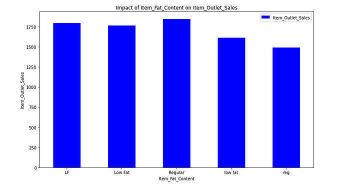
Low Fat products seem to higher sales than the Regular products

1.2.2.2. Impact of Outlet_Identifier on Item_Outlet_Sales

Outlet_Identifier_pivot = train.pivot_table(index='Outlet_Identifier', values="Item_Outlet_Sales", aggfunc=np.median)
Outlet_Identifier_pivot.plot(kind='bar', color='blue',figsize=(12,7))

plt.xlabel("Outlet_Identifier")
plt.ylabel("Item_Outlet_Sales")
plt.title("Impact of Outlet_Identifier on Item_Outlet_Sales")
plt.xticks(rotation=0)
plt.show()

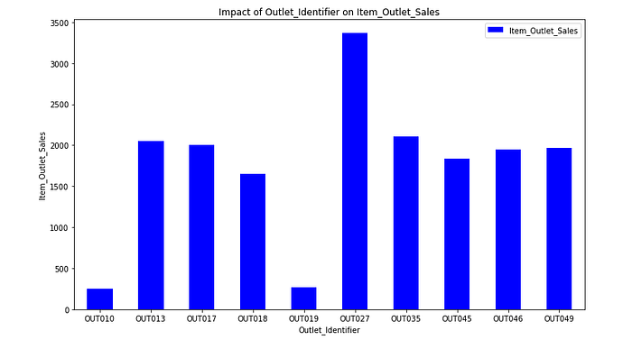
Out of 10- There are 2 Groceries strore, 6 Supermarket Type1, 1Supermarket Type2, and 1 Supermarket Type3. You can see from the below pivot table.

train.pivot_table(values='Outlet_Type',
              columns='Outlet_Identifier',
              aggfunc=lambda x:x.mode())

train.pivot_table(values='Outlet_Type',
              columns='Outlet_Size',
              aggfunc=lambda x:x.mode())

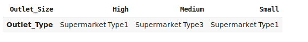
Most of the stores are of Supermarket Type1 of size High and they do not have best results. whereas Supermarket Type3 (OUT027) is a Medium size store and have best results.

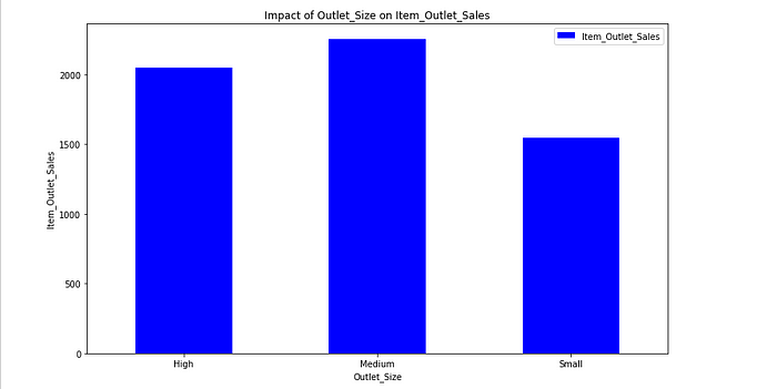
1.2.2.3. Impact of Outlet_Size on Item_Outlet_Sales

Outlet_Size_pivot = train.pivot_table(index='Outlet_Size', values="Item_Outlet_Sales", aggfunc=np.median)
Outlet_Size_pivot.plot(kind='bar', color='blue',figsize=(12,7))

plt.xlabel("Outlet_Size")
plt.ylabel("Item_Outlet_Sales")
plt.title("Impact of Outlet_Size on Item_Outlet_Sales")
plt.xticks(rotation=0)
plt.show()

1.2.2.4. Impact of Outlet_Type on Item_Outlet_Sales

Outlet_Type_pivot = train.pivot_table(index='Outlet_Type', values="Item_Outlet_Sales", aggfunc=np.median)
Outlet_Type_pivot.plot(kind='bar', color='blue',figsize=(12,7))

plt.xlabel("Outlet_Type")
plt.ylabel("Item_Outlet_Sales")
plt.title("Impact of Outlet_Size on Item_Outlet_Sales")
plt.xticks(rotation=0)
plt.show()

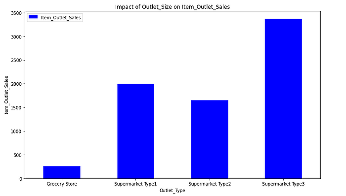
It could be a good idea to create a new feature that shows the sales ratio according to the store size.

1.2.2.5. Impact of Outlet_Location_Type on Item_Outlet_Sales

Outlet_Location_Type_pivot = train.pivot_table(index='Outlet_Location_Type', values="Item_Outlet_Sales", aggfunc=np.median)
Outlet_Location_Type_pivot.plot(kind='bar', color='blue',figsize=(12,7))

plt.xlabel("Outlet_Location_Type")
plt.ylabel("Item_Outlet_Sales")
plt.title("Impact of Outlet_Location_Type on Item_Outlet_Sales")
plt.xticks(rotation=0)
plt.show()

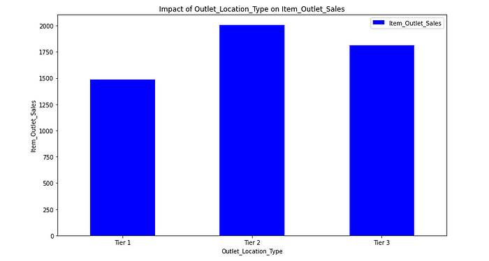
This shows that our hypotheses was totaly different from the result that we got from the above plot. Tier 2 cities have the higher sales than the Tier 1 and Tier 2.

train.pivot_table(values='Outlet_Location_Type',
              columns='Outlet_Type',
              aggfunc=lambda x:x.mode())

2. Data Pre-Processing

During our EDA we were able to take some Insights regarding our first hypotheses and the available data.

2. 1. Looking for missing values

We have two datasets the first one train.csv and the second is test.csv. Let's combine them into a dataframe data with a source column specifying where each observation belongs, so that we don't have to do pre-processing separately.

# Join Train and Test Dataset

#Create source column to later separate the data easily
train['source']='train'
test['source']='test'
data = pd.concat([train,test], ignore_index = True)
print(train.shape, test.shape, data.shape)

Now checking for the percentage of missing values present in our data:

data.isnull().sum()/data.shape[0]*100
#show values in percentage

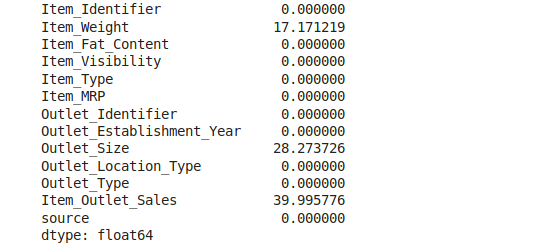
Note that Item_Outlet_Sales is the target variable and contains missing values because our test data does not have the Item_Outlet_Sales column.
Nevertheless, we'll impute the missing values in Item_Weight and Outlet_Size.

2.2. Imputing Missing Values In our EDA section, we have seen that the Item_Weight and the Outlet_Size had missing values.

In our EDA section, we have seen that the Item_Weight and the Outlet_Size had missing values.

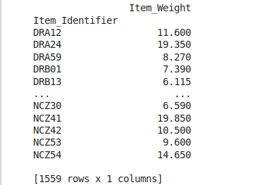
2.2.1. Imputing the mean for Item_Weight missing values

item_avg_weight = data.pivot_table(values='Item_Weight', index='Item_Identifier')
print(item_avg_weight)

def impute_weight(cols):
  Weight = cols[0]
  Identifier = cols[1]

  if pd.isnull(Weight):
    return item_avg_weight['Item_Weight'][item_avg_weight.index == Identifier]

  else:
    return Weight

print('Original #missing: %d'%sum(data['Item_Weight'].isnull()))

data['Item_Weight'] = data[['Item_Weight', 'Item_Identifier']].apply(impute_weight,axis=1).astype(float)

print('Final #missing: %d'%sum(data['Item_Weight'].isnull()))

2.2.2. Imputing Outlet_Size missing values with the mode

#Import mode function:
from scipy.stats import mode #Determing the mode for each
outlet_size_mode = data.pivot_table(values='Outlet_Size', columns='Outlet_Type',aggfunc=lambda x:x.mode())

outlet_size_mode

def impute_size_mode(cols):
    Size = cols[0]
    Type = cols[1]

    if pd.isnull(Size):
        return outlet_size_mode.loc['Outlet_Size']      [outlet_size_mode.columns == Type][0]
    else:
        return Size

print ('Orignal #missing: %d'%sum(data['Outlet_Size'].isnull()))

data['Outlet_Size'] = data[['Outlet_Size','Outlet_Type']].apply(impute_size_mode,axis=1)

print ('Final #missing: %d'%sum(data['Outlet_Size'].isnull()))

3. Feature Engineering

3.1. Should we combine Outlet_Type?

#Creates pivot table with Outlet_Type and the mean of
#Item_Outlet_Sales. Agg function is by default mean()

data.pivot_table(values='Item_Outlet_Sales', columns='Outlet_Type')

We are not going to combine because the average product sale are different.

3.2. Item_Visibility minimum value is 0

In our EDA we observe that Item_Visibility had minimum value 0. so this make no sense, lets consider it as missing value and impute with its mean.

#Determine average visibility of a productvisibility_avg = data.pivot_table(values='Item_Visibility', index='Item_Identifier')

#Impute 0 values with mean visibility of that productmissing_values = (data['Item_Visibility'] == 0)

print ('Number of 0 values initially: %d'%sum(missing_values))

data.loc[missing_values,'Item_Visibility'] = data.loc[missing_values,'Item_Identifier'].apply(lambda x: visibility_avg.at[x, 'Item_Visibility'])

print ('Number of 0 values after modification: %d'%sum(data['Item_Visibility'] == 0))

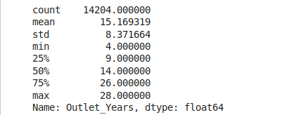
3.3. Determine the years of operation of a store

Data we have is from 2013, so we will create a new feature calculating the age of outlets.

#Remember the data is from 2013
data['Outlet_Years'] = 2013 - data['Outlet_Establishment_Year']
data['Outlet_Years'].describe()

3.4. Create a broad category of Item_Type

Item_Type is having 16 unique categories which might to be very useful in our analysis. So it's a good idea to combine them. Take a close look at Item_identifier each item starts with FD” (Food), “DR” (Drinks) or “NC” (Non-Consumables). We can group the items within these 3 categories.

#Get the first two characters of ID:data['Item_Type_Combined'] = data['Item_Identifier'].apply(lambda x: x[0:2])

#Rename them to more intuitive categories:data['Item_Type_Combined'] = data['Item_Type_Combined'].map({'FD':'Food','NC':'Non-Consumable',
          'DR':'Drinks'})data['Item_Type_Combined'].value_counts()

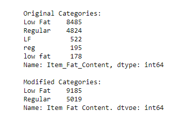
3.5. Modify categories of Item_Fat_Content

Here we are correcting the Typos in categories of Item_Fat_Content variable.

#Change the category of low fatprint('Original Categories:')
print(data['Item_Fat_Content'].value_counts())

print('\nModified categories')
data['Item_Fat_Content'] = data['Item_Fat_Content'].replace({'LF':'Low Fat',
                              'low fat':'Low Fat',
                              'reg':'Regular'})

print(data['Item_Fat_Content'].value_counts())

Wait, we have seen some non-consumables previously:

and a fat-content should not be specified for them. we will create a separate category for such kind observations.

#Mark non-consumables as separate category in low_fat:

data.loc[data['Item_Type_Combined'] ==
"Non-Consumable", "Item_Fat_Content"] = "Non-Edible"data['Item_Fat_Content'].value_counts()

BigMart Sales Prediction step by step tutorial ends here.

https://www.buymeacoffee.com/Inje

Connect with me on LinkedIn: Md Injemamul Irshad