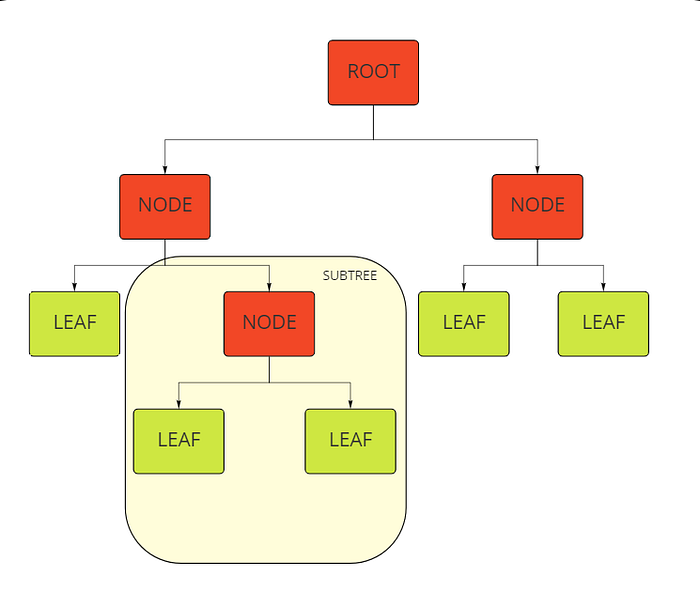
A decision tree has a flowchart structure, each feature is represented by an internal node, data is split by branches, and each leaf node represents the outcome. It is a white box, supervised machine learning algorithm, meaning all partitioning logic is accessible.
In this article, we will implement decision trees from the sklearn library and try to understand them through the parameters it takes.
Overfitting in Decision Trees
Overfitting is a serious problem in decision trees. Therefore, there are a lot of mechanisms to prune trees. Two main groups; pre-pruning is to stop the tree earlier. In post-pruning, we let the tree grow, and we check the overfitting status later and prune the tree if necessary. Cross-validation is used to test the need for pruning.
Firstly let's import the classification model from sklearn.
from sklearn.tree import DecisionTreeClassifier

#defaults
class sklearn.tree.DecisionTreeClassifier
(
*, criterion='gini', splitter='best', max_depth=None,
min_samples_split=2, min_samples_leaf=1, min_weight_fraction_leaf=0.0,
max_features=None, random_state=None, max_leaf_nodes=None,
min_impurity_decrease=0.0, class_weight=None, ccp_alpha=0.0
)
Criterion
{“gini”,”entropy”}, default = “gini”
Here we specify which method we will choose when performing split operations. Partition is the most important concept in decision trees. It is very crucial to determine how to split and when to split. To understand this better, we need to know some concepts.
Entropy
“Entropy increases. Things fall apart.” by John Green
Entropy is actually a very deep concept, a philosophical subject, and also a subject of thermodynamics. It is explained in the second law of thermodynamics in Britannica as follows:
The total entropy of an isolated system (the thermal energy per unit temperature that is unavailable for doing useful work) can never decrease.
From a very general perspective, we can define entropy as a measure of the disorder of a system. From this point of view, in our case, it is the measure of impurity in a split.
Entropy formula:
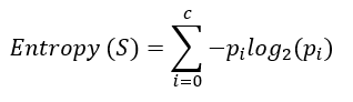
p is i-th class probability. Splitting with less entropy ensures optimum results.
We have one root node and two internal nodes in the following case. Each section has some “yes” (+) sample and some “no” (-) sample.
A sample tree:
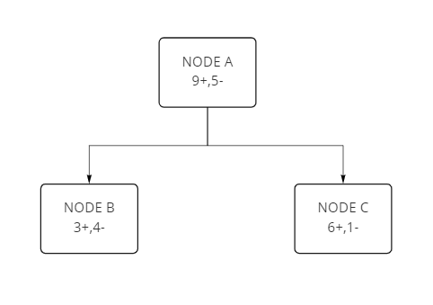
Let's calculate the entropy of Node A:
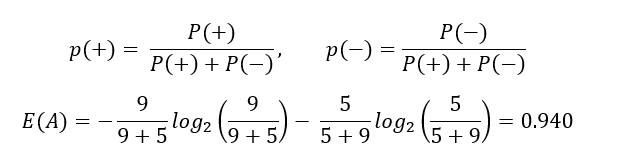
Entropy for each node:
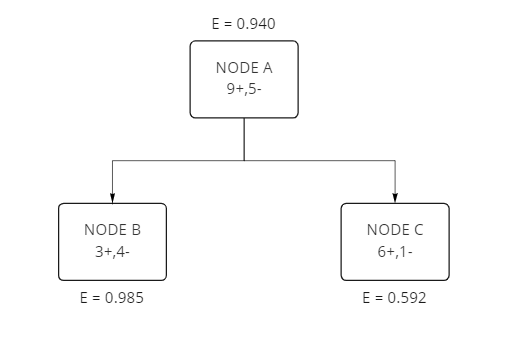
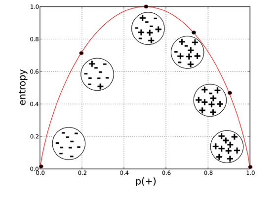
Entropy ranges from 0 to 1. If entropy is 0, consider it as a pure sub-tree and entropy becomes 1 if all labels are equally distributed in a leaf; in our case, it is 50%-50%. The entropy of Node B is quite close to 1 because it has almost 50% percent mixture of samples.
Provost, Foster; Fawcett, Tom. Data Science for Business: What You Need to Know about Data Mining and Data-Analytic Thinking
Information Gain
How can we use entropy when making the split decision? Information gain measures the quality of the split. Thanks to gain, we learn how much we have reduced the entropy when we make a split.
Information gain formula:
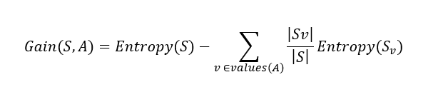
Now let's calculate the information gain in the split process above.
Gain (S,A) = 0.940-(7/14).0.985 - (7/14).592 = 0.151
Each time we choose the partitions with the higher information gain.
Gini Impurity
We can either use entropy or Gini impurity, they both measure the purity of a partition in a different mechanism.
Gini formula:
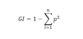
Let's calculate the Gini Impurity of Node C as an example:
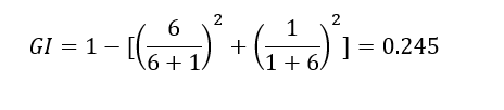
Entropy changes between 0 and 1, but Gini Impurity ranges between 0 and 0.5.
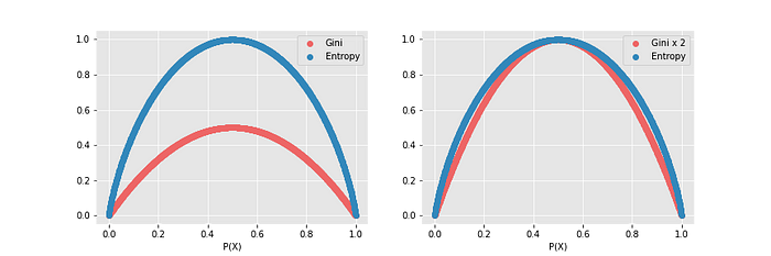
Computation power is reduced because the log function is not used in GI. Therefore, it will be solved faster than an entropy-used model. As can be seen from the second graph above, there is a slight difference between them. Therefore, GI may be preferred in cases where solving time is important.
splitter
{“best, “random”}, default = “best”
It is the strategy of how to split a node. The best splitter goes through all possible sets of splits on each feature in the dataset and selects the best split. It always gives the same result, it chooses the same feature and threshold to split because it always looks for the best split.
The random option adds randomness to the model, the split has been made between random subsets of features. It will traverse all the features the same as the best option, but will only select some features (defined in the max_features parameter) to compare information gained between them.
max_features
int, float or {“auto,”sqrt”,”log2"}, default=None
The number of features to consider when splitting. We can determine the maximum number of features to be used by giving integers and proportionally by giving float numbers. If a float is given, then max_features will be int(max_features * n_features). sqrt is the square root number of total features and log2 is the log2 of the total feature number.
By limiting the feature number, we are creating subsampling which is a way to decorrelate trees. Recommended default values are m = p/3 for regression and the square root of p for classification problems according to Elements of Statistical Learning.
max_depth
int, default = None
It determines the maximum depth of the tree. If None is given, then splitting continues until all leaves are all pure (or until it reaches the limit which is specified in the min_samples_split parameter). The hypothetical maximum number or depth would be number_of_training_sample-1, but tree algorithms always have a stopping mechanism that does not allow this.
Attempting to split all the way deeper will most likely result in overfitting. In the opposite situation, less depth may result in underfitting. Therefore, this is an important hyperparameter that needs to be thought about and perhaps should be tuned by trial and error. It should be evaluated in a specific way for each dataset, and problem.
min_samples_split
int or float, default = 2
It determines the minimum number of samples an internal node must have before it can be split. You can define it with an integer value, or you can set fractions by passing floats, ceil(min_sample_split*n_samples). Recall that, an internal node can be split further. This is another important parameter to regularize and control overfitting.
This parameter (and min_sample_leaf) is a defensive rule. It helps to stop tree growth.
min_samples_leaf
int or float, default = 1
It determines the minimum number of samples an external node (leaf) must have. Practically keep it between 1 to 20.
min_weight_fraction_leaf
float, default = 0
If you think some features in the dataset are more important and trustable than others, you can pass weights into the model, and by setting min_weight_fraction_leaf, leaves with lower weight sums will not be created in the first place.
random_state
int, RandomState instance or None, default = None
Seeding, setting the randomness.
max_leaf_nodes
int, default = None
Limit the maximum number of leaves in a tree.
min_impurity_decrease
float, default = 0.0
When evaluating every split alternative, how much impurity is reduced is calculated and the most contributing is selected for splitting. If we set min_impurity_decrease, then the model will use this value as a threshold before splitting. We can avoid unnecessary splits by telling the model how much of an improvement there is for meaningful splitting.
class_weight
dict, list of dict or “balanced”, default = None
You can assign a weight to each class. If you choose “balanced”, it will automatically assign a weight according to the frequency. Weights should be used in imbalanced datasets to label balancing. Practically, start with the “balanced” option and tune weights later by trial and error.
ccp_alpha
non-negative float, default = 0.0
Cost complexity pruning. It is another parameter to control the size of the tree. Larger values increase the number of nodes pruned.
Now let's apply a generic decision tree with sklearn in Python and then examine its attributes.
from sklearn.datasets import load_iris
from sklearn.tree import DecisionTreeClassifier

data = load_iris()
X = data.data
y = data.target
clf = DecisionTreeClassifier()
clf.fit(X,y)
Simple implementation of a decision tree on the iris dataset
Attributes
classes_: returns classes of the target.
print(clf.classes_)
#[0 1 2]
feature_importances_: the importance of each feature (Gini importance).
print(clf.feature_importances_)
#[0.02666667 0.         0.55072262 0.42261071]
max_features_ , n_classes_ , n_features_in_ , n_outputs_:
These return whatever they point to in their names.
print(clf.max_features_)
#4
print(clf.n_classes_)
#3
print(clf.n_features_in_)
#4
print(clf.n_outputs_)
#1
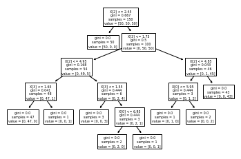
tree_: returns the tree object.
Visualization of tree
from sklearn import tree
tree.plot_tree(elf)
Conclusion
Decision Tree is a very popular tool for classification (or regression) problems. It provides clear indications to understand the importance of features, it is a white box. It is easier to make trial and error. On the other hand, it is very vulnerable to overfitting, not a robust model I think.
Frankly, I do not use decision trees directly, random forest is preferable in practice, but actually, it just means more than one tree.
That's it for this topic. Thank you for reading.
Comments
Loading comments…