In my previous article, I have highlighted 4 algorithms to start off in Machine Learning: Linear Regression, Logistic Regression, Decision Trees and Random Forest. Now, I am creating a series of the same.
The equation which defines the simplest form of the regression equation with one dependent and one independent variable: y = mx+c.
Where y = estimated dependent variable, c = constant, m= regression coefficient and x = independent variable.
Let's just understand with an example:
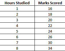
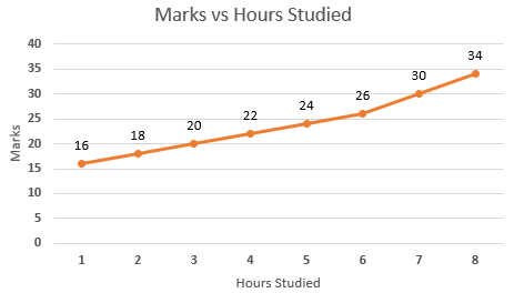
Hours vs Marks Scored by the Students
Say; There is a certain relationship between the marks scored by the students (y- Dependent variable) in an exam and hours they studied for the exam(x- Independent Variable). Now we want to predict the marks scored by the students by input the hours studied. Here, x would be the input and y would be the output. Linear regression model would predict the marks of the students when the user will input the number of hours studied.
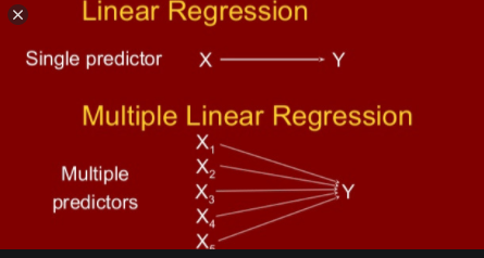
That is just a simple example of Linear regression, Linear Regression can be divided into two types:
- Simple Linear Regression: If a single independent variable is used to predict the value of a numerical dependent variable, then such a Linear Regression algorithm is called Simple Linear Regression.
- Multiple Linear Regression: If more than one independent variable is used to predict the value of a numerical dependent variable, then such a Linear Regression algorithm is called Multiple Linear Regression.
Assessing Goodness-of-Fit in a Regression Model
R-Squared: It evaluates the scatter of the data points around the fitted regression line. We also call it the coefficient of determination, or the coefficient of multiple determination for multiple regression. It measures the strength of the relationship between the dependent and independent variables on a scale of 0–100%.
To visually show how R-Squared values represent the scatter around the regression line, you can plot the fitted values by observed values.
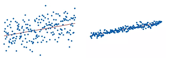
The R-squared for the regression model on the left is 15%, and for the model on the right it is 85%. When a regression model accounts for more of the variance, the data points are closer to the regression line. You’ll never see a regression model with an R2 of 100%. In that case, the fitted values equal the data values and, all the observations fall exactly on the regression line.
R-Squared has Limitations
You cannot use R-Squared to determine whether it biases the coefficient estimates and predictions, which is why you must assess the residual plots.
R-Squared does not show if a regression model provides an adequate fit to your data. A suitable model can have a low R2 value. On the other hand, a biased model can have a high R2 value.
Assumption of Linear Regression
- Linear relationship between the features and target.
- Small or no multicollinearity between the features: Multicollinearity means high-correlation between the independent variables. Because of multicollinearity, it may difficult to find the true relationship between the predictors and target variables.
- Homoscedasticity: variance of the residual, or error term, in a regression model is constant.
- No autocorrelations: Autocorrelation usually occurs if there is a dependency between residual errors.
Conclusion
Honestly, there is still lots of information around Linear regression but this will give you the fair idea about the Linear Regression.
Hope it helps you to kick-start your Machine Learning Journey.
Happy Learning!
Comments
Loading comments…