Mapping Elevation Data in Python’s Matplotlib

STEP 1 : Get the elevation data

In order to plot the 3D terrain — commonly refered to as “elevation” in the geographers’ field — we first need to acquire this data from a trusted source. Many websites can give you such information, with various degrees of accuracy, and among them is the United State’s Geological Survey’s Earth Explorer, which will perfectly match our needs in this case.

USGS’s Earth Explorer Website:

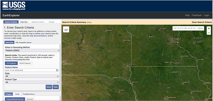
In order to find the data of interest, go to the Data Sets section in the left hand-side menu, and select the GTOPO30 option. On a side note, this elevation map is not the most precise, and covers the globe using large tiles, which do not provide good data for very small scales. However, they are largely sufficient for most usecases, as we will resize and crop the image data as we like.

Dataset selection:

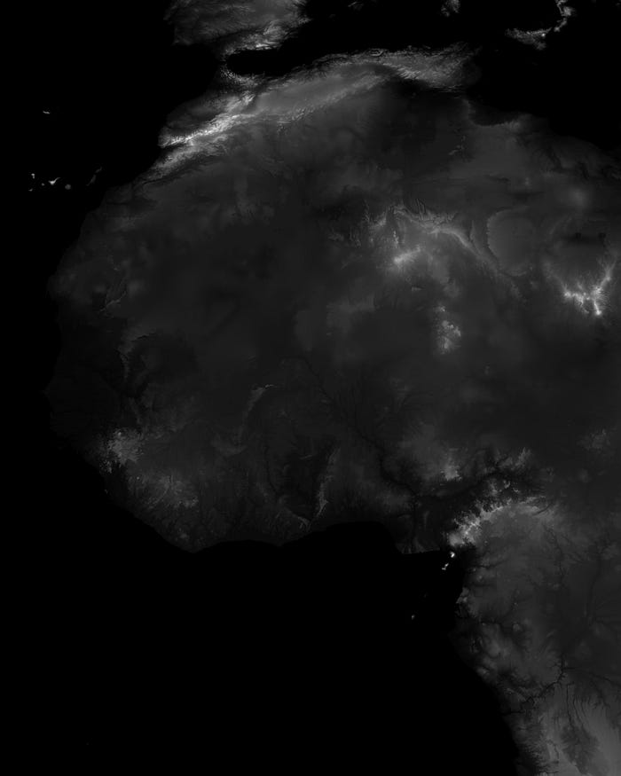
Next, find the elevation data picture that encompasses the land you would like to map. Note that the tiles are named after the latitude and longitude they cover. For this exemple, we will use the North-West African Tile (GT30W020N40) as to get both mountains and oceans to make this look interesting.

North-West Africa Tile, GT30W020N40:

STEP 2 : Get the python script ready

We first import all the necessary packages : PIL.Image to load and resize/crop the picture, Numpy to deal with the picture’s data and a subset of matplotlib’s libraries to plot nicely the result.

import numpy as np  
import matplotlib.pyplot as plt  
from matplotlib.colors import LinearSegmentedColormap, ListedColormap  
from matplotlib import cm  
from PIL import Image

Then we’ll add some lines to get a custom color map from the “terrain” default map, that will differentiate between land (elevation above 1m) and water (yes, you guessed it, below 1m). In a few words, this piece of code firstly loads the “terrain” color map (you can find more matplotlib color maps here), samples it from 20% of the spectrum to the end (to cut off the blue color and save it for the ocean), and finally adds the blue RGB values at the beginning of the spectrum, before declaring it as a new usable color map.

terrain = cm.get_cmap("terrain").resampled(256)  
newcolors = terrain(np.linspace(0.2, 1, 256))  
newcolors[:1, :] = np.array([39/256, 30/256, 100/256, 1])  
newcmp = ListedColormap(newcolors)

STEP 3: Make the plotting function

In order to be able to plot from any data picture, we’ll define a function map. In the first lines of the function, we take the image from the file path input (always make sure the path has the backslashes “\” escaped as “\”) and we crop it to one interesting part (note that 1° of latitude or longitude is represented by 120 pixels in the picture, which is why i use multiples of 120).

Then, we use some numpy magic to define the plotting grid, using our reduction parameter : set to 1, you get full details (might crash or slow down your computer noticeably for big areas) — set to 10, you divide by 10 the number of sample points in your picture, and so on for bigger values. One may also decrease the detail level of the plot by increasing the rstride and cstride values in the plot_surface function. The exageration input is used to increase the height of the surface’s features for a more dramatic effect.

def map(path,reduction=10,exageration=4):  
    img = Image.open(path) #MAKE SURE THE "\" ARE ESCAPED AS "\\" IN THE PATH !  
    img = img.crop((10*120,5*120,15*120,10*120)) #CROP TO YOUR DESIRED SPOT HERE !  
    x,y = img.size  
    img = np.flipud(exageration*np.asarray(img.resize((int(x/reduction),int(y/reduction))),dtype=int))  
    X,Y = np.meshgrid(np.linspace(0,int(x/reduction),int(x/reduction)),np.linspace(0,int(y/reduction),int(y/reduction)))  
    ax = plt.figure().add_subplot(projection='3d')  
    ax.set_zlim([0,5000])  
    ax.plot_surface(X,Y,img,rstride=1,cstride=1,alpha=1,cmap=newcmp,antialiased=False)  
    plt.show()

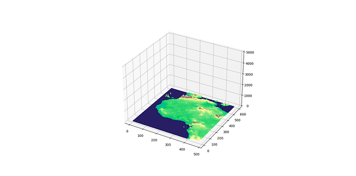
STEP 4: Enjoy

Once our function is ready, we can now get a clean elevation plot in two lines of code:

file_path = "C:\\Users\\Username\\Pictures\\gt30w020n40.jpg"  
  
map(file_path,reduction=15,exageration=2)

Here are a few results you can get from this setup, varying the inputs :

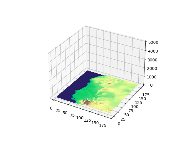
1. Varying the localisation (cropping)

Different croping values, exageration=4 & reduction=10:

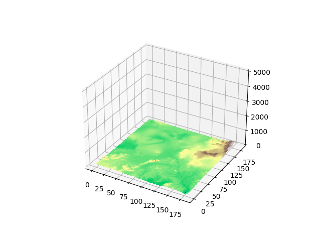
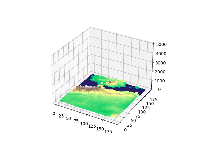
2. Varying the reduction

Different reduction values (100;30;10), exageration=4:

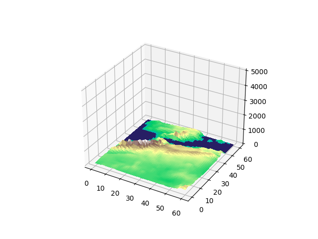
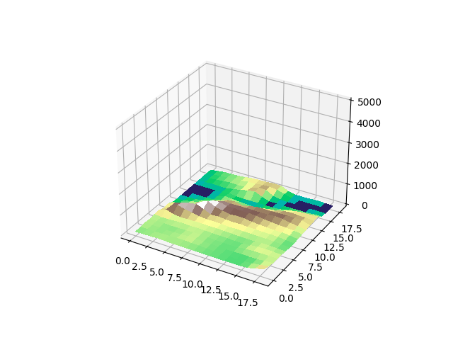
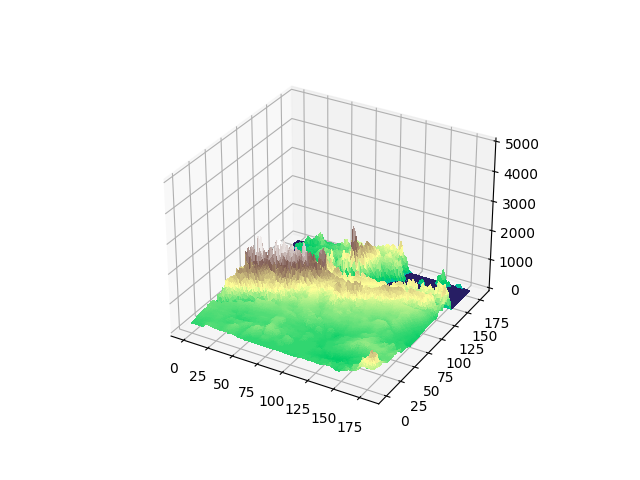
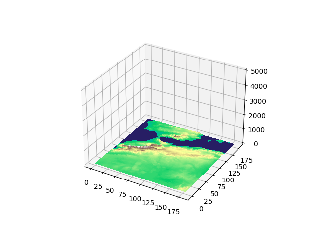
3. Varying the exageration

Different exageration values (1;4;10):

Here’s the full code in case you need a quick copy/paste:

import numpy as np  
import matplotlib.pyplot as plt  
from matplotlib.colors import LinearSegmentedColormap, ListedColormap  
from matplotlib import cm  
from PIL import Image  
  
terrain = cm.get_cmap("terrain").resampled(256)  
newcolors = terrain(np.linspace(0.2, 1, 256))  
newcolors[:1, :] = np.array([39/256, 30/256, 100/256, 1])  
newcmp = ListedColormap(newcolors)  
  
def map(path,reduction=10,exageration=4):  
    img = Image.open(path) #MAKE SURE THE "\" ARE ESCAPED AS "\\" IN THE PATH !  
    img = img.crop((10*120,5*120,15*120,10*120)) #CROP TO YOUR DESIRED SPOT HERE !  
    x,y = img.size  
    img = np.flipud(exageration*np.asarray(img.resize((int(x/reduction),int(y/reduction))),dtype=int))  
    X,Y = np.meshgrid(np.linspace(0,int(x/reduction),int(x/reduction)),np.linspace(0,int(y/reduction),int(y/reduction)))  
    ax = plt.figure().add_subplot(projection='3d')  
    ax.set_zlim([0,5000])  
    ax.plot_surface(X, Y,img,rstride=1, cstride=1,alpha=1,cmap=newcmp,antialiased=False)  
    plt.show()  
  
file_path = "C:\\Users\\Username\\Pictures\\gt30w020n40.jpg"  
  
map(file_path,reduction=15,exageration=2)

Thank you for reading!