This helps to address some of the problems associated with vanilla gradient descent, such as oscillations, slow convergence, and getting stuck in local minima.
The fundamental intuition behind momentum-based gradient descent is the concept of momentum in physics. A classic and simple example is a ball rolling down a hill that gathers enough momentum to overcome a plateau region and make it to a global minimum instead of getting stuck at a local minimum. Momentum adds history to the parameter updates of descent problems which significantly accelerates the optimization process.
The amount of history included in the update equation is determined by a hyperparameter. This hyperparameter is a value ranging from 0 to 1, where a momentum value of 0 is equivalent to gradient descent without momentum. A higher momentum value means more gradients from the past (history) are considered.
Problems with gradient descent
Let’s start with outlining some of the problems that afflict vanilla gradient descent algorithms.
- Local Minima
Gradient descent can get stuck in local minima, points that are not the global minimum of the cost function but are still lower than the surrounding points. This can occur when the cost function has multiple valleys, and the algorithm gets stuck in one instead of reaching the global minimum as illustrated below:
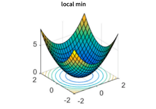 ALL images created by author
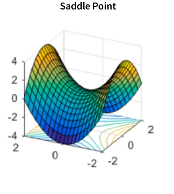
2. Saddle Points
A saddle point is a point in the cost function where one dimension has a higher value than the surrounding points, and the other has a lower value. Gradient descent can get stuck at these points because the gradients in one direction point towards a lower value, while those in the other direction point towards a higher value.
3. Plateaus
A plateau is a region in the cost function where the gradients are very small or close to zero. This can cause gradient descent to take a long time or not converge.

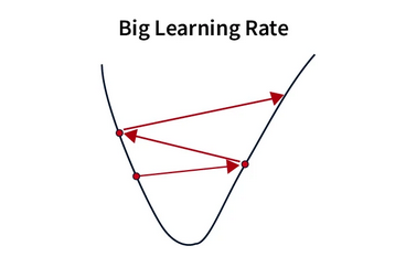
4. Oscillations
Oscillations occur when the learning rate is too high, causing the algorithm to overshoot the minimum and oscillate back and forth.
Gradient descent is subject to several other difficulties, among the most notable and extensively discussed being vanishing gradients and exploding gradients.
How Momentum-based gradient descent works
After examining the problems with gradient descent and hence the motivations to come up with enhancements and improvements, let’s move on to discussing how gradient descent actually works. This will require only some basic algebra and will be explained along the way with plain English.
The fundamental expression for regular gradient descent looks as follows:
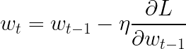
Here, w_t is the weight at the current time step, w_{t-1} is the weight at the previous time step, η is the learning rate and the last term is the partial derivative of the loss function with respect to the weight at previous step (aka gradient).
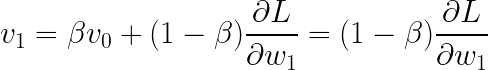
Now, we must include a term for momentum and revise the updating equation to account for the new hyperparameter and momentum.
Here, V_t is defined as:

This equation is referred to as an** exponentially weighted average.** β is our momentum hyperparameter. When β = 0, the equation is the same as vanilla gradient descent.
We start out with V_0 = 0 and update the equation for t= 1…n.

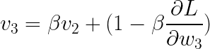
substituting:

simplifying:

Now,
substituting:
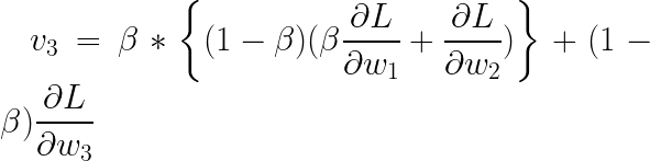
simplifying:

generalizing:

The generalized summation includes all previous gradients that have been built up through all iterations.
The hyperparameter Beta
Now the question is what do we set the new hyperparameter β to.
If we set it to a low value, e.g. 0.1, then the gradient at t=3 will contribute 100% of its value, the gradient at t=2 will contribute 10% of its value, and the gradient at t=1 will only contribute 1% of its value. You can see that the contributions from earlier gradients decreases rapidly if we set β too low.
If, on the other hand, we set a high value for β, say 0.9, the gradient at t=3 will contribute 100% of its value, the gradient at t=2 will contribute 90% of its value, and the gradient at t=1 will contribute 81% of its value.
We conclude that a higher β will include more gradients from the past. This is what is meant by momentum and how it builds up throughout the process.
Implementation in Python with NumPy
Here is an implementation of Gradient Descent with Momentum along with a step-by-step explanation and output comparison to Vanilla Gradient Descent.
Before diving into the implementation, let’s understand the difference between Vanilla Gradient Descent and Gradient Descent with Momentum:
Vanilla Gradient Descent: 1. Compute the gradient of the loss function with respect to the parameters. 2. Update the parameters by subtracting a small fraction (learning rate) of the gradient’s magnitude from the current parameter values. 3. Repeat steps 1 and 2 until convergence is reached.
Gradient Descent with Momentum: 1. Compute the gradient of the loss function with respect to the parameters. 2. Calculate an exponentially weighted moving average (momentum) of the gradients from step 1. 3. Update the parameters by modifying the update step in Vanilla Gradient Descent with the momentum term. 4. Repeat steps 1–3 until convergence is reached.
Now, let’s go through the implementation:
import numpy as np

def gradient_descent_momentum(X, y, learning_rate=0.01, momentum=0.9, num_iterations=100):
    # Initialize the parameters
    num_samples, num_features = X.shape
    theta = np.zeros(num_features)

    # Initialize the velocity vector
    velocity = np.zeros_like(theta)

    # Perform iterations
    for iteration in range(num_iterations):
        # Compute the predictions and errors
        predicted = np.dot(X, theta)
        errors = predicted - y

        # Compute the gradients
        gradients = (1/num_samples) * np.dot(X.T, errors)

        # Update the velocity
        velocity = momentum * velocity + learning_rate * gradients

        # Update the parameters
        theta -= velocity

        # Compute the mean squared error
        mse = np.mean(errors**2)

        # Print the MSE at each iteration
        print(f"Iteration {iteration+1}, MSE: {mse}")

    return theta
Now, let’s compare the output of Gradient Descent with Momentum to Vanilla Gradient Descent using a simple linear regression problem:
# Generate some random data
np.random.seed(42)
X = np.random.rand(100, 1)
y = 2 + 3 * X + np.random.randn(100, 1)

# Apply Gradient Descent with Momentum
theta_momentum = gradient_descent_momentum(X, y, learning_rate=0.1, momentum=0.9, num_iterations=100)

# Apply Vanilla Gradient Descent
theta_vanilla = gradient_descent(X, y, learning_rate=0.1, num_iterations=100)
Output:
Iteration 1, MSE: 5.894802675477298
Iteration 2, MSE: 4.981474209682729
Iteration 3, MSE: 4.543813739311503
...
Iteration 98, MSE: 0.639280357661573
Iteration 99, MSE: 0.6389711476228525
Iteration 100, MSE: 0.63867258334531

Iteration 1, MSE: 5.894802675477298
Iteration 2, MSE: 4.981474209682729
Iteration 3, MSE: 4.543813739311503
...
Iteration 98, MSE: 0.639280357661573
Iteration 99, MSE: 0.6389711476228525
Iteration 100, MSE: 0.63867258334531
As we can see from the output, both Gradient Descent with Momentum and Vanilla Gradient Descent provide similar results. However, Gradient Descent with Momentum can converge faster due to the momentum term, which accelerates the updates in the direction of the most recent gradients, leading to faster convergence.
Applications
Momentum is widely used in the machine learning community for optimizing non-convex functions such as deep neural networks. Empirically, momentum methods outperform traditional stochastic gradient descent approaches. In deep learning, SGD is widely prevalent and is the underlying basis for many optimizers such as Adam, Adadelta, RMSProp, etc. which already utilize momentum to reduce computation speed
The momentum extension for optimization algorithms is available in many popular machine learning frameworks such as PyTorch, tensor flow, and scikit-learn. Generally, any problem that can be solved with stochastic gradient descent can benefit from the application of momentum. These are often unconstrained optimization problems. Some common SGD applications where momentum may be applied are ridge and logistic regression and support vector machines.Classification problems including those relating to cancer diagnosis and image determination can also have reduced run times when momentum is implemented. In the case of medical diagnoses, this increased computation speed can directly benefit patients through faster diagnosis times and higher accuracy of diagnosis within the neural network.
Summary
Momentum improves on gradient descent by reducing oscillatory effects and acting as an accelerator for optimization problem solving. Additionally, it finds the global (and not just local) optimum. Because of these advantages, momentum is commonly used in machine learning and has broad applications to all optimizers through SGD. Though the hyperparameters for momentum must be chosen with care and requires some trial and error, it ultimately addresses common issues seen in gradient descent problems. As deep learning continues to advance, momentum application will allow models and problems to be trained and solved faster than methods without.
References
Brownlee, J. (2021, October 11). Gradient descent with momentum from scratch. Machine Learning Mastery. https://machinelearningmastery.com/gradient-descent-with-momentum-from-scratch/.
Sum, C. -S. Leung and K. Ho, “A Limitation of Gradient Descent Learning,” in IEEE Transactions on Neural Networks and Learning Systems, vol. 31, no. 6, pp. 2227–2232, June 2020, doi: 10.1109/TNNLS.2019.2927689
Srihari, S. (n.d.). Basic Optimization Algorithms. Deep learning.https://cedar.buffalo.edu/~srihari/CSE676/8.3%20BasicOptimizn.pdf
Comments
Loading comments…