A Transformer lighting up a dark cave with a torch. Generated with Dall•E 3.

Note: This article is an excerpt of my latest Notebook, Transformer From Scratch With PyTorch🔥 | Kaggle

Introduction

In 2017, the Google Research team published a paper called “Attention Is All You Need”, which presented the Transformer architecture and was a paradigm shift in Machine Learning, especially in Deep Learning and the field of natural language processing.

The Transformer, with its parallel processing capabilities, allowed for more efficient and scalable models, making it easier to train them on large datasets. It also demonstrated superior performance in several NLP tasks, such as sentiment analysis and text generation tasks.

The archicture presented in this paper served as the foundation for subsequent models like GPT and BERT. Besides NLP, the Transformer architecture is used in other fields, like audio processing and computer vision. You can see the usage of Transformers in audio classification in the notebook Audio Data: Music Genre Classification.

Even though you can easily employ different types of Transformers with the 🤗Transformers library, it is crucial to understand how things truly work by building them from scratch.

In this notebook, we will explore the Transformer architecture and all its components. I will use PyTorch to build all the necessary structures and blocks, and I will use the Coding a Transformer from scratch on PyTorch, with full explanation, training and inference video posted by Umar Jamil on YouTube as reference.

Let’s start by importing all the necessary libraries.

# Importing libraries

# PyTorch
import torch
import torch.nn as nn
from torch.utils.data import Dataset, DataLoader, random_split
from torch.utils.tensorboard import SummaryWriter

# Math
import math

# HuggingFace libraries
from datasets import load_dataset
from tokenizers import Tokenizer
from tokenizers.models import WordLevel
from tokenizers.trainers import WordLevelTrainer
from tokenizers.pre_tokenizers import Whitespace

# Pathlib
from pathlib import Path

# typing
from typing import  Any

# Library for progress bars in loops
from tqdm import tqdm

# Importing library of warnings
import warnings

Transformer Architecture

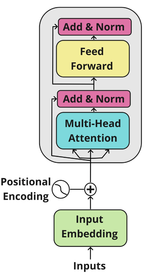
Before coding, let’s take a look at the Transformer architecture.

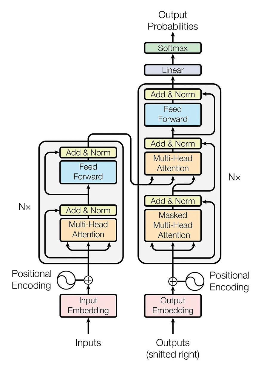
Source: Attention Is All You Need

The Transformer architecture has two main blocks: the encoder and the decoder. Let’s take a look at them further.

Encoder: It has a Multi-Head Attention mechanism and a fully connected Feed-Forward network. There are also residual connections around the two sub-layers, plus layer normalization for the output of each sub-layer. All sub-layers in the model and the embedding layers produce outputs of dimension 𝑑𝑚𝑜𝑑𝑒𝑙=512_.

Decoder: The decoder follows a similar structure, but it inserts a third sub-layer that performs multi-head attention over the output of the encoder block. There is also a modification of the self-attention sub-layer in the decoder block to avoid positions from attending to subsequent positions. This masking ensures that the predictions for position 𝑖 depend solely on the known outputs at positions less than 𝑖.

Both the encoder and decode blocks are repeated 𝑁 times. In the original paper, they defined 𝑁 = 6, and we will define a similar value in this notebook.

Input Embeddings

When we observe the Transformer architecture image above, we can see that the Embeddings represent the first step of both blocks.

The InputEmbedding class below is responsible for converting the input text into numerical vectors of d_model dimensions. To prevent that our input embeddings become extremely small, we normalize them by multiplying them by the √𝑑𝑚𝑜𝑑𝑒𝑙_

In the image below, we can see how the embeddings are created. First, we have a sentence that gets split into tokens — we will explore what tokens are later on — . Then, the token IDs — identification numbers — are transformed into the embeddings, which are high-dimensional vectors.

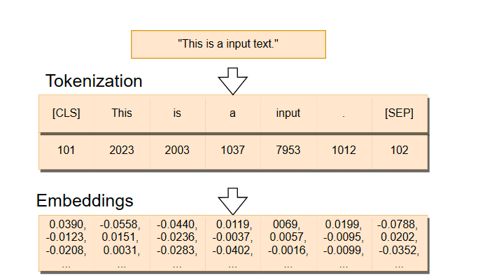
Tokenization and Embeddings. Source: vaclavkosar.com

# Creating Input Embeddings
class  InputEmbeddings(nn.Module):

def  __init__(self, d_model: int, vocab_size: int):
super().__init__()
self.d_model = d_model # Dimension of vectors (512)
self.vocab_size = vocab_size # Size of the vocabulary
self.embedding = nn.Embedding(vocab_size, d_model) # PyTorch layer that converts integer indices to dense embeddings

def  forward(self, x):
return self.embedding(x) * math.sqrt(self.d_model) # Normalizing the variance of the embeddings

Positional Encoding

In the original paper, the authors add the positional encodings to the input embeddings at the bottom of both the encoder and decoder blocks so the model can have some information about the relative or absolute position of the tokens in the sequence. The positional encodings have the same dimension 𝑑_model the embeddings, so that the two vectors can be summed and we can combine the semantic content from the word embeddings and positional information from the positional encodings.

In the PositionalEncoding class below, we will create a matrix of positional encodings pe with dimensions (seq_len, d_model). We will start by filling it with 0s.We will then apply the sine function to even indices of the positional encoding matrix while the cosine function is applied to the odd ones.

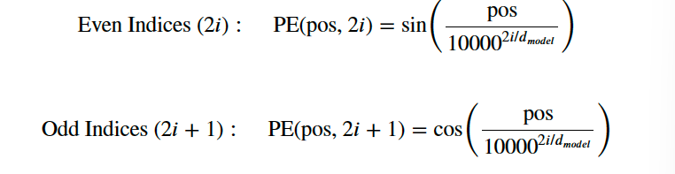
Positional encoding formulas.Source: Attention Is All You Need

We apply the sine and cosine functions because it allows the model to determine the position of a word based on the position of other words in the sequence, since for any fixed offset 𝑘, 𝑃𝐸ₚₒₛ ₊ ₖcan be represented as a linear function of 𝑃𝐸ₚₒₛ. This happens due to the properties of sine and cosine functions, where a shift in the input results in a predictable change in the output.

# Creating the Positional Encoding
class  PositionalEncoding(nn.Module):

def  __init__(self, d_model: int, seq_len: int, dropout: float) -> None:
super().__init__()
self.d_model = d_model # Dimensionality of the model
self.seq_len = seq_len # Maximum sequence length
self.dropout = nn.Dropout(dropout) # Dropout layer to prevent overfitting

# Creating a positional encoding matrix of shape (seq_len, d_model) filled with zeros
pe = torch.zeros(seq_len, d_model)

# Creating a tensor representing positions (0 to seq_len - 1)
position = torch.arange(0, seq_len, dtype = torch.float).unsqueeze(1) # Transforming 'position' into a 2D tensor['seq_len, 1']

# Creating the division term for the positional encoding formula
div_term = torch.exp(torch.arange(0, d_model, 2).float() * (-math.log(10000.0) / d_model))

# Apply sine to even indices in pe
pe[:, 0::2] = torch.sin(position * div_term)
# Apply cosine to odd indices in pe
pe[:, 1::2] = torch.cos(position * div_term)

# Adding an extra dimension at the beginning of pe matrix for batch handling
pe = pe.unsqueeze(0)

# Registering 'pe' as buffer. Buffer is a tensor not considered as a model parameter
self.register_buffer('pe', pe)

def  forward(self,x):
# Addind positional encoding to the input tensor X
x = x + (self.pe[:, :x.shape[1], :]).requires_grad_(False)
return self.dropout(x) # Dropout for regularization

Layer Normalization

When we look at the encoder and decoder blocks, we see several normalization layers called Add & Norm.

The LayerNormalization class below performs layer normalization on the input data. During its forward pass, we compute the mean and standard deviation of the input data. We then normalize the input data by subtracting the mean and dividing by the standard deviation plus a small number called epsilon to avoid any divisions by zero. This process results in a normalized output with a mean 0 and a standard deviation 1.

We will then scale the normalized output by a learnable parameter alpha and add a learnable parameter called bias. The training process is responsible for adjusting these parameters. The final result is a layer-normalized tensor, which ensures that the scale of the inputs to layers in the network is consistent.

# Creating Layer Normalization
class  LayerNormalization(nn.Module):

def  __init__(self, eps: float = 10**-6) -> None: # We define epsilon as 0.000001 to avoid division by zero
super().__init__()
self.eps = eps

# We define alpha as a trainable parameter and initialize it with ones
self.alpha = nn.Parameter(torch.ones(1)) # One-dimensional tensor that will be used to scale the input data

# We define bias as a trainable parameter and initialize it with zeros
self.bias = nn.Parameter(torch.zeros(1)) # One-dimensional tenso that will be added to the input data

def  forward(self, x):
mean = x.mean(dim = -1, keepdim = True) # Computing the mean of the input data. Keeping the number of dimensions unchanged
std = x.std(dim = -1, keepdim = True) # Computing the standard deviation of the input data. Keeping the number of dimensions unchanged

# Returning the normalized input
return self.alpha * (x-mean) / (std + self.eps) + self.bias

Feed-Forward Network

In the fully connected feed-forward network, we apply two linear transformations with a ReLU activation in between. We can mathematically represent this operation as:

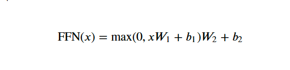
Source: Attention Is All You Need

W₁ and W₂ are the weights, while b₁ and b₂ are the biases of the two linear transformations.

In the FeedForwardBlock below, we will define the two linear transformations—self.linear_1 and self.linear_2—and the inner-layer d_ff. The input data will first pass through the self.linear_1 transformation, which increases its dimensionality from d_model to d_ff. The output of this operation passes through the ReLU activation function, which introduces non-linearity so the network can learn more complex patterns, and the self.dropout layer is applied to mitigate overfitting. The final operation is the self.linear_2 transformation to the dropout-modified tensor, which transforms it back to the original d_model dimension.

# Creating Feed Forward Layers
class  FeedForwardBlock(nn.Module):

def  __init__(self, d_model: int, d_ff: int, dropout: float) -> None:
super().__init__()
# First linear transformation
self.linear_1 = nn.Linear(d_model, d_ff) # W1 & b1
self.dropout = nn.Dropout(dropout) # Dropout to prevent overfitting
# Second linear transformation
self.linear_2 = nn.Linear(d_ff, d_model) # W2 & b2

def  forward(self, x):
# (Batch, seq_len, d_model) --> (batch, seq_len, d_ff) -->(batch, seq_len, d_model)
return self.linear_2(self.dropout(torch.relu(self.linear_1(x))))

Multi-Head Attention

he Multi-Head Attention is the most crucial component of the Transformer. It is responsible for helping the model to understand complex relationships and patterns in the data.

The image below displays how the Multi-Head Attention works. It doesn’t include batch dimension because it only illustrates the process for one single sentence.

Source: YouTube: Coding a Transformer from scratch on PyTorch, with full explanation, training and inference by Umar Jamil.

The Multi-Head Attention block receives the input data split into queries, keys, and values organized into matrices 𝑄, 𝐾, and 𝑉. Each matrix contains different facets of the input, and they have the same dimensions as the input.

We then linearly transform each matrix by their respective weight matrices 𝑊^Q, 𝑊^K, and 𝑊^V. These transformations will result in new matrices 𝑄′, 𝐾′, and 𝑉′, which will be split into smaller matrices corresponding to different heads ℎ, allowing the model to attend to information from different representation subspaces in parallel. This split creates multiple sets of queries, keys, and values for each head.

Finally, we concatenate every head into an 𝐻 matrix, which is then transformed by another weight matrix 𝑊𝑜 to produce the multi-head attention output, a matrix 𝑀𝐻−𝐴 that retains the input dimensionality.

# Creating the Multi-Head Attention block
class  MultiHeadAttentionBlock(nn.Module):

def  __init__(self, d_model: int, h: int, dropout: float) -> None: # h = number of heads
super().__init__()
self.d_model = d_model
self.h = h

# We ensure that the dimensions of the model is divisible by the number of heads
assert d_model % h == 0, 'd_model is not divisible by h'

# d_k is the dimension of each attention head's key, query, and value vectors
self.d_k = d_model // h # d_k formula, like in the original "Attention Is All You Need" paper

# Defining the weight matrices
self.w_q = nn.Linear(d_model, d_model) # W_q
self.w_k = nn.Linear(d_model, d_model) # W_k
self.w_v = nn.Linear(d_model, d_model) # W_v
self.w_o = nn.Linear(d_model, d_model) # W_o

self.dropout = nn.Dropout(dropout) # Dropout layer to avoid overfitting


@staticmethod
def  attention(query, key, value, mask, dropout: nn.Dropout):# mask => When we want certain words to NOT interact with others, we "hide" them

d_k = query.shape[-1] # The last dimension of query, key, and value

# We calculate the Attention(Q,K,V) as in the formula in the image above
attention_scores = (query @ key.transpose(-2,-1)) / math.sqrt(d_k) # @ = Matrix multiplication sign in PyTorch

# Before applying the softmax, we apply the mask to hide some interactions between words
if mask is  not  None: # If a mask IS defined...
attention_scores.masked_fill_(mask == 0, -1e9) # Replace each value where mask is equal to 0 by -1e9
attention_scores = attention_scores.softmax(dim = -1) # Applying softmax
if dropout is  not  None: # If a dropout IS defined...
attention_scores = dropout(attention_scores) # We apply dropout to prevent overfitting

return (attention_scores @ value), attention_scores # Multiply the output matrix by the V matrix, as in the formula

def  forward(self, q, k, v, mask):

query = self.w_q(q) # Q' matrix
key = self.w_k(k) # K' matrix
value = self.w_v(v) # V' matrix


# Splitting results into smaller matrices for the different heads
# Splitting embeddings (third dimension) into h parts
query = query.view(query.shape[0], query.shape[1], self.h, self.d_k).transpose(1,2) # Transpose => bring the head to the second dimension
key = key.view(key.shape[0], key.shape[1], self.h, self.d_k).transpose(1,2) # Transpose => bring the head to the second dimension
value = value.view(value.shape[0], value.shape[1], self.h, self.d_k).transpose(1,2) # Transpose => bring the head to the second dimension

# Obtaining the output and the attention scores
x, self.attention_scores = MultiHeadAttentionBlock.attention(query, key, value, mask, self.dropout)

# Obtaining the H matrix
x = x.transpose(1, 2).contiguous().view(x.shape[0], -1, self.h * self.d_k)

return self.w_o(x) # Multiply the H matrix by the weight matrix W_o, resulting in the MH-A matrix

Residual Connection

When we look at the architecture of the Transformer, we see that each sub-layer, including the self-attention and Feed Forward blocks, adds its output to its input before passing it to the Add & Norm layer. This approach integrates the output with the original input in the Add & Norm layer. This process is known as the skip connection, which allows the Transformer to train deep networks more effectively by providing a shortcut for the gradient to flow through during backpropagation.

The ResidualConnection class below is responsible for this process.

# Building Residual Connection
class  ResidualConnection(nn.Module):
def  __init__(self, dropout: float) -> None:
super().__init__()
self.dropout = nn.Dropout(dropout) # We use a dropout layer to prevent overfitting
self.norm = LayerNormalization() # We use a normalization layer

def  forward(self, x, sublayer):
# We normalize the input and add it to the original input 'x'. This creates the residual connection process.
return x + self.dropout(sublayer(self.norm(x)))

Encoder

We will now build the encoder. We create the EncoderBlock class, consisting of the Multi-Head Attention and Feed Forward layers, plus the residual connections.

Encoder block. Source: researchgate.net.

In the original paper, the Encoder Block repeats six times. We create the Encoder class as an assembly of multiple EncoderBlocks. We also add layer normalization as a final step after processing the input through all its blocks.

# Building Encoder Block
class  EncoderBlock(nn.Module):

# This block takes in the MultiHeadAttentionBlock and FeedForwardBlock, as well as the dropout rate for the residual connections
def  __init__(self, self_attention_block: MultiHeadAttentionBlock, feed_forward_block: FeedForwardBlock, dropout: float) -> None:
super().__init__()
# Storing the self-attention block and feed-forward block
self.self_attention_block = self_attention_block
self.feed_forward_block = feed_forward_block
self.residual_connections = nn.ModuleList([ResidualConnection(dropout) for _ in  range(2)]) # 2 Residual Connections with dropout

def  forward(self, x, src_mask):
# Applying the first residual connection with the self-attention block
x = self.residual_connections[0](x, lambda x: self.self_attention_block(x, x, x, src_mask)) # Three 'x's corresponding to query, key, and value inputs plus source mask

# Applying the second residual connection with the feed-forward block
x = self.residual_connections[1](x, self.feed_forward_block)
return x # Output tensor after applying self-attention and feed-forward layers with residual connections.

# Building Encoder
# An Encoder can have several Encoder Blocks
class  Encoder(nn.Module):

# The Encoder takes in instances of 'EncoderBlock'
def  __init__(self, layers: nn.ModuleList) -> None:
super().__init__()
self.layers = layers # Storing the EncoderBlocks
self.norm = LayerNormalization() # Layer for the normalization of the output of the encoder layers

def  forward(self, x, mask):
# Iterating over each EncoderBlock stored in self.layers
for layer in self.layers:
x = layer(x, mask) # Applying each EncoderBlock to the input tensor 'x'
return self.norm(x) # Normalizing output

Decoder

Similarly, the Decoder also consists of several DecoderBlocks that repeat six times in the original paper. The main difference is that it has an additional sub-layer that performs multi-head attention with a cross-attention component that uses the output of the Encoder as its keys and values while using the Decoder’s input as queries.

Decoder block. Source: edlitera.com.

For the Output Embedding, we can use the same InputEmbeddings class we use for the Encoder. You can also notice that the self-attention sub-layer is masked, which restricts the model from accessing future elements in the sequence.

We will start by building the DecoderBlock class, and then we will build the Decoder class, which will assemble multiple DecoderBlocks.

# Building Decoder Block
class  DecoderBlock(nn.Module):

# The DecoderBlock takes in two MultiHeadAttentionBlock. One is self-attention, while the other is cross-attention.
# It also takes in the feed-forward block and the dropout rate
def  __init__(self, self_attention_block: MultiHeadAttentionBlock, cross_attention_block: MultiHeadAttentionBlock, feed_forward_block: FeedForwardBlock, dropout: float) -> None:
super().__init__()
self.self_attention_block = self_attention_block
self.cross_attention_block = cross_attention_block
self.feed_forward_block = feed_forward_block
self.residual_connections = nn.ModuleList([ResidualConnection(dropout) for _ in  range(3)]) # List of three Residual Connections with dropout rate

def  forward(self, x, encoder_output, src_mask, tgt_mask):

# Self-Attention block with query, key, and value plus the target language mask
x = self.residual_connections[0](x, lambda x: self.self_attention_block(x, x, x, tgt_mask))

# The Cross-Attention block using two 'encoder_ouput's for key and value plus the source language mask. It also takes in 'x' for Decoder queries
x = self.residual_connections[1](x, lambda x: self.cross_attention_block(x, encoder_output, encoder_output, src_mask))

# Feed-forward block with residual connections
x = self.residual_connections[2](x, self.feed_forward_block)
return x

# Building Decoder
# A Decoder can have several Decoder Blocks
class  Decoder(nn.Module):

# The Decoder takes in instances of 'DecoderBlock'
def  __init__(self, layers: nn.ModuleList) -> None:
super().__init__()

# Storing the 'DecoderBlock's
self.layers = layers
self.norm = LayerNormalization() # Layer to normalize the output

def  forward(self, x, encoder_output, src_mask, tgt_mask):

# Iterating over each DecoderBlock stored in self.layers
for layer in self.layers:
# Applies each DecoderBlock to the input 'x' plus the encoder output and source and target masks
x = layer(x, encoder_output, src_mask, tgt_mask)
return self.norm(x) # Returns normalized output

You can see in the Decoder image that after running a stack of DecoderBlocks, we have a Linear Layer and a Softmax function to the output of probabilities. The ProjectionLayer class below is responsible for converting the output of the model into a probability distribution over the vocabulary, where we select each output token from a vocabulary of possible tokens.

# Buiding Linear Layer
class  ProjectionLayer(nn.Module):
def  __init__(self, d_model: int, vocab_size: int) -> None: # Model dimension and the size of the output vocabulary
super().__init__()
self.proj = nn.Linear(d_model, vocab_size) # Linear layer for projecting the feature space of 'd_model' to the output space of 'vocab_size'
def  forward(self, x):
return torch.log_softmax(self.proj(x), dim = -1) # Applying the log Softmax function to the output

Building the Transformer

We finally have every component of the Transformer architecture ready. We may now construct the Transformer by putting it all together.

In the Transformer class below, we will bring together all the components of the model's architecture.

# Creating the Transformer Architecture
class  Transformer(nn.Module):

# This takes in the encoder and decoder, as well the embeddings for the source and target language.
# It also takes in the Positional Encoding for the source and target language, as well as the projection layer
def  __init__(self, encoder: Encoder, decoder: Decoder, src_embed: InputEmbeddings, tgt_embed: InputEmbeddings, src_pos: PositionalEncoding, tgt_pos: PositionalEncoding, projection_layer: ProjectionLayer) -> None:
super().__init__()
self.encoder = encoder
self.decoder = decoder
self.src_embed = src_embed
self.tgt_embed = tgt_embed
self.src_pos = src_pos
self.tgt_pos = tgt_pos
self.projection_layer = projection_layer

# Encoder
def  encode(self, src, src_mask):
src = self.src_embed(src) # Applying source embeddings to the input source language
src = self.src_pos(src) # Applying source positional encoding to the source embeddings
return self.encoder(src, src_mask) # Returning the source embeddings plus a source mask to prevent attention to certain elements

# Decoder
def  decode(self, encoder_output, src_mask, tgt, tgt_mask):
tgt = self.tgt_embed(tgt) # Applying target embeddings to the input target language (tgt)
tgt = self.tgt_pos(tgt) # Applying target positional encoding to the target embeddings

# Returning the target embeddings, the output of the encoder, and both source and target masks
# The target mask ensures that the model won't 'see' future elements of the sequence
return self.decoder(tgt, encoder_output, src_mask, tgt_mask)

# Applying Projection Layer with the Softmax function to the Decoder output
def  project(self, x):
return self.projection_layer(x)

The architecture is finally ready. We now define a function called build_transformer, in which we define the parameters and everything we need to have a fully operational Transformer model for the task of machine translation.

We will set the same parameters as in the original paper, Attention Is All You Need, where 𝑑𝑚𝑜𝑑𝑒𝑙 = 512_, 𝑁 = 6, ℎ = 8, dropout rate 𝑃𝑑𝑟𝑜𝑝 = 0.1_, and 𝑑𝑓𝑓= 2048_.

# Building & Initializing Transformer

# Definin function and its parameter, including model dimension, number of encoder and decoder stacks, heads, etc.
def  build_transformer(src_vocab_size: int, tgt_vocab_size: int, src_seq_len: int, tgt_seq_len: int, d_model: int = 512, N: int = 6, h: int = 8, dropout: float = 0.1, d_ff: int = 2048) -> Transformer:

# Creating Embedding layers
src_embed = InputEmbeddings(d_model, src_vocab_size) # Source language (Source Vocabulary to 512-dimensional vectors)
tgt_embed = InputEmbeddings(d_model, tgt_vocab_size) # Target language (Target Vocabulary to 512-dimensional vectors)

# Creating Positional Encoding layers
src_pos = PositionalEncoding(d_model, src_seq_len, dropout) # Positional encoding for the source language embeddings
tgt_pos = PositionalEncoding(d_model, tgt_seq_len, dropout) # Positional encoding for the target language embeddings

# Creating EncoderBlocks
encoder_blocks = [] # Initial list of empty EncoderBlocks
for _ in  range(N): # Iterating 'N' times to create 'N' EncoderBlocks (N = 6)
encoder_self_attention_block = MultiHeadAttentionBlock(d_model, h, dropout) # Self-Attention
feed_forward_block = FeedForwardBlock(d_model, d_ff, dropout) # FeedForward

# Combine layers into an EncoderBlock
encoder_block = EncoderBlock(encoder_self_attention_block, feed_forward_block, dropout)
encoder_blocks.append(encoder_block) # Appending EncoderBlock to the list of EncoderBlocks

# Creating DecoderBlocks
decoder_blocks = [] # Initial list of empty DecoderBlocks
for _ in  range(N): # Iterating 'N' times to create 'N' DecoderBlocks (N = 6)
decoder_self_attention_block = MultiHeadAttentionBlock(d_model, h, dropout) # Self-Attention
decoder_cross_attention_block = MultiHeadAttentionBlock(d_model, h, dropout) # Cross-Attention
feed_forward_block = FeedForwardBlock(d_model, d_ff, dropout) # FeedForward

# Combining layers into a DecoderBlock
decoder_block = DecoderBlock(decoder_self_attention_block, decoder_cross_attention_block, feed_forward_block, dropout)
decoder_blocks.append(decoder_block) # Appending DecoderBlock to the list of DecoderBlocks

# Creating the Encoder and Decoder by using the EncoderBlocks and DecoderBlocks lists
encoder = Encoder(nn.ModuleList(encoder_blocks))
decoder = Decoder(nn.ModuleList(decoder_blocks))

# Creating projection layer
projection_layer = ProjectionLayer(d_model, tgt_vocab_size) # Map the output of Decoder to the Target Vocabulary Space

# Creating the transformer by combining everything above
transformer = Transformer(encoder, decoder, src_embed, tgt_embed, src_pos, tgt_pos, projection_layer)

# Initialize the parameters
for p in transformer.parameters():
if p.dim() > 1:
nn.init.xavier_uniform_(p)

return transformer # Assembled and initialized Transformer. Ready to be trained and validated!

The model is now ready to be trained!

Tokenizer

Tokenization is a crucial preprocessing step for our Transformer model. In this step, we convert raw text into a number format that the model can process.

There are several Tokenization strategies. We will use the word-level tokenization to transform each word in a sentence into a token.

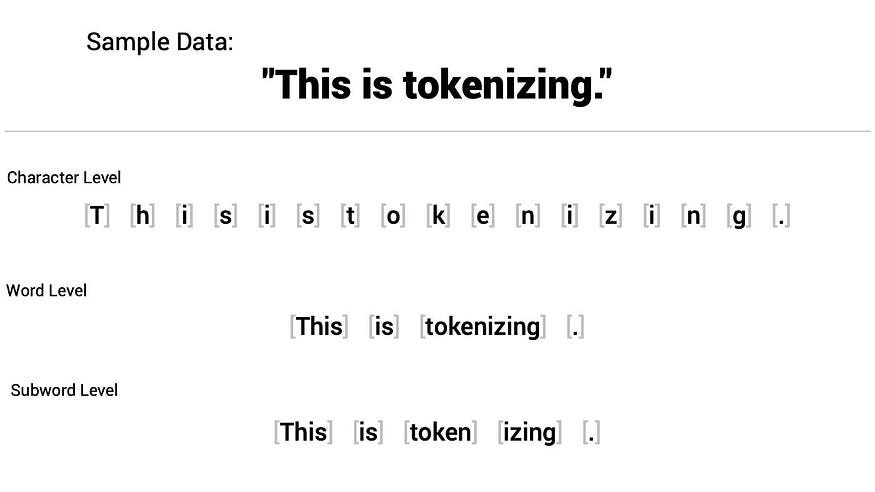
Different tokenization strategies. Source: shaankhosla.substack.com.

After tokenizing a sentence, we map each token to an unique integer ID based on the created vocabulary present in the training corpus during the training of the tokenizer. Each integer number represents a specific word in the vocabulary.

Besides the words in the training corpus, Transformers use special tokens for specific purposes. These are some that we will define right away:

• [UNK]: This token is used to identify an unknown word in the sequence.

• [PAD]: Padding token to ensure that all sequences in a batch have the same length, so we pad shorter sentences with this token. We use attention masks to “tell” the model to ignore the padded tokens during training since they don’t have any real meaning to the task.

• [SOS]: This is a token used to signal the Start of Sentence.

• [EOS]: This is a token used to signal the End of Sentence.

In the build_tokenizer function below, we ensure a tokenizer is ready to train the model. It checks if there is an existing tokenizer, and if that is not the case, it trains a new tokenizer.

# Defining Tokenizer
def  build_tokenizer(config, ds, lang):

# Crating a file path for the tokenizer
tokenizer_path = Path(config['tokenizer_file'].format(lang))

# Checking if Tokenizer already exists
if  not Path.exists(tokenizer_path):

# If it doesn't exist, we create a new one
tokenizer = Tokenizer(WordLevel(unk_token = '[UNK]')) # Initializing a new world-level tokenizer
tokenizer.pre_tokenizer = Whitespace() # We will split the text into tokens based on whitespace

# Creating a trainer for the new tokenizer
trainer = WordLevelTrainer(special_tokens = ["[UNK]", "[PAD]",
"[SOS]", "[EOS]"], min_frequency = 2) # Defining Word Level strategy and special tokens

# Training new tokenizer on sentences from the dataset and language specified
tokenizer.train_from_iterator(get_all_sentences(ds, lang), trainer = trainer)
tokenizer.save(str(tokenizer_path)) # Saving trained tokenizer to the file path specified at the beginning of the function
else:
tokenizer = Tokenizer.from_file(str(tokenizer_path)) # If the tokenizer already exist, we load it
return tokenizer # Returns the loaded tokenizer or the trained tokenizer

Loading Dataset

For this task, we will use the OpusBooks dataset, available on 🤗Hugging Face. This dataset consists of two features, id and translation. The translation feature contains pairs of sentences in different languages, such as Spanish and Portuguese, English and French, and so forth.

I first tried translating sentences from English to Portuguese — my native tongue — but there are only 1.4k examples for this pair, so the results were not satisfying in the current configurations for this model. I then tried to use the English-French pair due to its higher number of examples — 127k — but it would take too long to train with the current configurations. I then opted to train the model on the English-Italian pair, the same one used in the Coding a Transformer from scratch on PyTorch, with full explanation, training and inference video, as that was a good balance between performance and time of training.

We start by defining the get_all_sentences function to iterate over the dataset and extract the sentences according to the language pair defined—we will do that later.

# Iterating through dataset to extract the original sentence and its translation
def  get_all_sentences(ds, lang):
for pair in ds:
yield pair['translation'][lang]

The get_ds function is defined to load and prepare the dataset for training and validation. In this function, we build or load the tokenizer, split the dataset, and create DataLoaders, so the model can successfully iterate over the dataset in batches. The result of these functions is tokenizers for the source and target languages plus the DataLoader objects.

def  get_ds(config):

# Loading the train portion of the OpusBooks dataset.
# The Language pairs will be defined in the 'config' dictionary we will build later
ds_raw = load_dataset('opus_books', f'{config["lang_src"]}-{config["lang_tgt"]}', split = 'train')

# Building or loading tokenizer for both the source and target languages
tokenizer_src = build_tokenizer(config, ds_raw, config['lang_src'])
tokenizer_tgt = build_tokenizer(config, ds_raw, config['lang_tgt'])

# Splitting the dataset for training and validation
train_ds_size = int(0.9 * len(ds_raw)) # 90% for training
val_ds_size = len(ds_raw) - train_ds_size # 10% for validation
train_ds_raw, val_ds_raw = random_split(ds_raw, [train_ds_size, val_ds_size]) # Randomly splitting the dataset

# Processing data with the BilingualDataset class, which we will define below
train_ds = BilingualDataset(train_ds_raw, tokenizer_src, tokenizer_tgt, config['lang_src'], config['lang_tgt'], config['seq_len'])
val_ds = BilingualDataset(val_ds_raw, tokenizer_src, tokenizer_tgt, config['lang_src'], config['lang_tgt'], config['seq_len'])

# Iterating over the entire dataset and printing the maximum length found in the sentences of both the source and target languages
max_len_src = 0
max_len_tgt = 0
for pair in ds_raw:
src_ids = tokenizer_src.encode(pair['translation'][config['lang_src']]).ids
tgt_ids = tokenizer_src.encode(pair['translation'][config['lang_tgt']]).ids
max_len_src = max(max_len_src, len(src_ids))
max_len_tgt = max(max_len_tgt, len(tgt_ids))

print(f'Max length of source sentence: {max_len_src}')
print(f'Max length of target sentence: {max_len_tgt}')

# Creating dataloaders for the training and validadion sets
# Dataloaders are used to iterate over the dataset in batches during training and validation
train_dataloader = DataLoader(train_ds, batch_size = config['batch_size'], shuffle = True) # Batch size will be defined in the config dictionary
val_dataloader = DataLoader(val_ds, batch_size = 1, shuffle = True)

return train_dataloader, val_dataloader, tokenizer_src, tokenizer_tgt # Returning the DataLoader objects and tokenizers

We define the casual_mask function to create a mask for the attention mechanism of the decoder. This mask prevents the model from having information about future elements in the sequence.

We start by making a square grid filled with ones. We determine the grid size with the size parameter. Then, we change all the numbers above the main diagonal line to zeros. Every number on one side becomes a zero, while the rest remain ones. The function then flips all these values, turning ones into zeros and zeros into ones. This process is crucial for models that predict future tokens in a sequence.

def  casual_mask(size):
# Creating a square matrix of dimensions 'size x size' filled with ones
mask = torch.triu(torch.ones(1, size, size), diagonal = 1).type(torch.int)
return mask == 0

The BilingualDataset class processes the texts of the target and source languages in the dataset by tokenizing them and adding all the necessary special tokens. This class also certifies that the sentences are within a maximum sequence length for both languages and pads all necessary sentences.

class  BilingualDataset(Dataset):

# This takes in the dataset contaning sentence pairs, the tokenizers for target and source languages, and the strings of source and target languages
# 'seq_len' defines the sequence length for both languages
def  __init__(self, ds, tokenizer_src, tokenizer_tgt, src_lang, tgt_lang, seq_len) -> None:
super().__init__()

self.seq_len = seq_len
self.ds = ds
self.tokenizer_src = tokenizer_src
self.tokenizer_tgt = tokenizer_tgt
self.src_lang = src_lang
self.tgt_lang = tgt_lang

# Defining special tokens by using the target language tokenizer
self.sos_token = torch.tensor([tokenizer_tgt.token_to_id("[SOS]")], dtype=torch.int64)
self.eos_token = torch.tensor([tokenizer_tgt.token_to_id("[EOS]")], dtype=torch.int64)
self.pad_token = torch.tensor([tokenizer_tgt.token_to_id("[PAD]")], dtype=torch.int64)


# Total number of instances in the dataset (some pairs are larger than others)
def  __len__(self):
return  len(self.ds)

# Using the index to retrive source and target texts
def  __getitem__(self, index: Any) -> Any:
src_target_pair = self.ds[index]
src_text = src_target_pair['translation'][self.src_lang]
tgt_text = src_target_pair['translation'][self.tgt_lang]

# Tokenizing source and target texts
enc_input_tokens = self.tokenizer_src.encode(src_text).ids
dec_input_tokens = self.tokenizer_tgt.encode(tgt_text).ids

# Computing how many padding tokens need to be added to the tokenized texts
# Source tokens
enc_num_padding_tokens = self.seq_len - len(enc_input_tokens) - 2  # Subtracting the two '[EOS]' and '[SOS]' special tokens
# Target tokens
dec_num_padding_tokens = self.seq_len - len(dec_input_tokens) - 1  # Subtracting the '[SOS]' special token

# If the texts exceed the 'seq_len' allowed, it will raise an error. This means that one of the sentences in the pair is too long to be processed
# given the current sequence length limit (this will be defined in the config dictionary below)
if enc_num_padding_tokens < 0  or dec_num_padding_tokens < 0:
raise ValueError('Sentence is too long')

# Building the encoder input tensor by combining several elements
encoder_input = torch.cat(
[
self.sos_token, # inserting the '[SOS]' token
torch.tensor(enc_input_tokens, dtype = torch.int64), # Inserting the tokenized source text
self.eos_token, # Inserting the '[EOS]' token
torch.tensor([self.pad_token] * enc_num_padding_tokens, dtype = torch.int64) # Addind padding tokens
]
)

# Building the decoder input tensor by combining several elements
decoder_input = torch.cat(
[
self.sos_token, # inserting the '[SOS]' token
torch.tensor(dec_input_tokens, dtype = torch.int64), # Inserting the tokenized target text
torch.tensor([self.pad_token] * dec_num_padding_tokens, dtype = torch.int64) # Addind padding tokens
]

)

# Creating a label tensor, the expected output for training the model
label = torch.cat(
[
torch.tensor(dec_input_tokens, dtype = torch.int64), # Inserting the tokenized target text
self.eos_token, # Inserting the '[EOS]' token
torch.tensor([self.pad_token] * dec_num_padding_tokens, dtype = torch.int64) # Adding padding tokens

]
)

# Ensuring that the length of each tensor above is equal to the defined 'seq_len'
assert encoder_input.size(0) == self.seq_len
assert decoder_input.size(0) == self.seq_len
assert label.size(0) == self.seq_len

return {
'encoder_input': encoder_input,
'decoder_input': decoder_input,
'encoder_mask': (encoder_input != self.pad_token).unsqueeze(0).unsqueeze(0).int(),
'decoder_mask': (decoder_input != self.pad_token).unsqueeze(0).unsqueeze(0).int() & casual_mask(decoder_input.size(0)),
'label': label,
'src_text': src_text,
'tgt_text': tgt_text
}

Validation Loop

We will now create two functions for the validation loop. The validation loop is crucial to evaluate model performance in translating sentences from data it has not seen during training.

We will define two functions. The first function, greedy_decode, gives us the model's output by obtaining the most probable next token. The second function, run_validation, is responsible for running the validation process in which we decode the model's output and compare it with the reference text for the target sentence.

# Define function to obtain the most probable next token
def  greedy_decode(model, source, source_mask, tokenizer_src, tokenizer_tgt, max_len, device):
# Retrieving the indices from the start and end of sequences of the target tokens
sos_idx = tokenizer_tgt.token_to_id('[SOS]')
eos_idx = tokenizer_tgt.token_to_id('[EOS]')

# Computing the output of the encoder for the source sequence
encoder_output = model.encode(source, source_mask)
# Initializing the decoder input with the Start of Sentence token
decoder_input = torch.empty(1,1).fill_(sos_idx).type_as(source).to(device)

# Looping until the 'max_len', maximum length, is reached
while  True:
if decoder_input.size(1) == max_len:
break

# Building a mask for the decoder input
decoder_mask = casual_mask(decoder_input.size(1)).type_as(source_mask).to(device)

# Calculating the output of the decoder
out = model.decode(encoder_output, source_mask, decoder_input, decoder_mask)

# Applying the projection layer to get the probabilities for the next token
prob = model.project(out[:, -1])

# Selecting token with the highest probability
_, next_word = torch.max(prob, dim=1)
decoder_input = torch.cat([decoder_input, torch.empty(1,1). type_as(source).fill_(next_word.item()).to(device)], dim=1)

# If the next token is an End of Sentence token, we finish the loop
if next_word == eos_idx:
break

return decoder_input.squeeze(0) # Sequence of tokens generated by the decoder

# Defining function to evaluate the model on the validation dataset
# num_examples = 2, two examples per run
def  run_validation(model, validation_ds, tokenizer_src, tokenizer_tgt, max_len, device, print_msg, global_state, writer, num_examples=2):
model.eval() # Setting model to evaluation mode
count = 0  # Initializing counter to keep track of how many examples have been processed

console_width = 80  # Fixed witdh for printed messages

# Creating evaluation loop
with torch.no_grad(): # Ensuring that no gradients are computed during this process
for batch in validation_ds:
count += 1
encoder_input = batch['encoder_input'].to(device)
encoder_mask = batch['encoder_mask'].to(device)

# Ensuring that the batch_size of the validation set is 1
assert encoder_input.size(0) == 1, 'Batch size must be 1 for validation.'

# Applying the 'greedy_decode' function to get the model's output for the source text of the input batch
model_out = greedy_decode(model, encoder_input, encoder_mask, tokenizer_src, tokenizer_tgt, max_len, device)

# Retrieving source and target texts from the batch
source_text = batch['src_text'][0]
target_text = batch['tgt_text'][0] # True translation
model_out_text = tokenizer_tgt.decode(model_out.detach().cpu().numpy()) # Decoded, human-readable model output

# Printing results
print_msg('-'*console_width)
print_msg(f'SOURCE: {source_text}')
print_msg(f'TARGET: {target_text}')
print_msg(f'PREDICTED: {model_out_text}')

# After two examples, we break the loop
if count == num_examples:
break

Training Loop

We are ready to train our Transformer model on the OpusBook dataset for the English to Italian translation task.

We first start by defining the get_model function to load the model by calling the build_transformer function we have previously defined. This function uses the config dictionary to set a few parameters.

# We pass as parameters the config dictionary, the length of the vocabylary of the source language and the target language
def  get_model(config, vocab_src_len, vocab_tgt_len):

# Loading model using the 'build_transformer' function.
# We will use the lengths of the source language and target language vocabularies, the 'seq_len', and the dimensionality of the embeddings
model = build_transformer(vocab_src_len, vocab_tgt_len, config['seq_len'], config['seq_len'], config['d_model'])
return model

I have mentioned the config dictionary several times throughout this notebook. Now, it is time to create it.

In the following cell, we will define two functions to configure our model and the training process.

In the get_config function, we define crucial parameters for the training process. batch_size for the number of training examples used in one iteration, num_epochs as the number of times the entire dataset is passed forward and backward through the Transformer, lr as the learning rate for the optimizer, etc. We will also finally define the pairs from the OpusBook dataset, 'lang_src': 'en' for selecting English as the source language and 'lang_tgt': 'it' for selecting Italian as the target language.

The get_weights_file_path function constructs the file path for saving or loading model weights for any specific epoch.

# Define settings for building and training the transformer model
def  get_config():
return{
'batch_size': 8,
'num_epochs': 20,
'lr': 10**-4,
'seq_len': 350,
'd_model': 512, # Dimensions of the embeddings in the Transformer. 512 like in the "Attention Is All You Need" paper.
'lang_src': 'en',
'lang_tgt': 'it',
'model_folder': 'weights',
'model_basename': 'tmodel_',
'preload': None,
'tokenizer_file': 'tokenizer_{0}.json',
'experiment_name': 'runs/tmodel'
}

# Function to construct the path for saving and retrieving model weights
def  get_weights_file_path(config, epoch: str):
model_folder = config['model_folder'] # Extracting model folder from the config
model_basename = config['model_basename'] # Extracting the base name for model files
model_filename = f"{model_basename}{epoch}.pt"  # Building filename
return  str(Path('.')/ model_folder/ model_filename) # Combining current directory, the model folder, and the model filename

We finally define our last function, train_model, which takes the config arguments as input.

In this function, we will set everything up for the training. We will load the model and its necessary components onto the GPU for faster training, set the Adam optimizer, and configure the CrossEntropyLoss function to compute the differences between the translations output by the model and the reference translations from the dataset.

Every loop necessary for iterating over the training batches, performing backpropagation, and computing the gradients is in this function. We will also use it to run the validation function and save the current state of the model.

def  train_model(config):
# Setting up device to run on GPU to train faster
device = torch.device('cuda'  if torch.cuda.is_available() else  'cpu')
print(f"Using device {device}")

# Creating model directory to store weights
Path(config['model_folder']).mkdir(parents=True, exist_ok=True)

# Retrieving dataloaders and tokenizers for source and target languages using the 'get_ds' function
train_dataloader, val_dataloader, tokenizer_src, tokenizer_tgt = get_ds(config)

# Initializing model on the GPU using the 'get_model' function
model = get_model(config,tokenizer_src.get_vocab_size(), tokenizer_tgt.get_vocab_size()).to(device)

# Tensorboard
writer = SummaryWriter(config['experiment_name'])

# Setting up the Adam optimizer with the specified learning rate from the '
# config' dictionary plus an epsilon value
optimizer = torch.optim.Adam(model.parameters(), lr=config['lr'], eps = 1e-9)

# Initializing epoch and global step variables
initial_epoch = 0
global_step = 0

# Checking if there is a pre-trained model to load
# If true, loads it
if config['preload']:
model_filename = get_weights_file_path(config, config['preload'])
print(f'Preloading model {model_filename}')
state = torch.load(model_filename) # Loading model

# Sets epoch to the saved in the state plus one, to resume from where it stopped
initial_epoch = state['epoch'] + 1
# Loading the optimizer state from the saved model
optimizer.load_state_dict(state['optimizer_state_dict'])
# Loading the global step state from the saved model
global_step = state['global_step']

# Initializing CrossEntropyLoss function for training
# We ignore padding tokens when computing loss, as they are not relevant for the learning process
# We also apply label_smoothing to prevent overfitting
loss_fn = nn.CrossEntropyLoss(ignore_index = tokenizer_src.token_to_id('[PAD]'), label_smoothing = 0.1).to(device)

# Initializing training loop

# Iterating over each epoch from the 'initial_epoch' variable up to
# the number of epochs informed in the config
for epoch in  range(initial_epoch, config['num_epochs']):

# Initializing an iterator over the training dataloader
# We also use tqdm to display a progress bar
batch_iterator = tqdm(train_dataloader, desc = f'Processing epoch {epoch:02d}')

# For each batch...
for batch in batch_iterator:
model.train() # Train the model

# Loading input data and masks onto the GPU
encoder_input = batch['encoder_input'].to(device)
decoder_input = batch['decoder_input'].to(device)
encoder_mask = batch['encoder_mask'].to(device)
decoder_mask = batch['decoder_mask'].to(device)

# Running tensors through the Transformer
encoder_output = model.encode(encoder_input, encoder_mask)
decoder_output = model.decode(encoder_output, encoder_mask, decoder_input, decoder_mask)
proj_output = model.project(decoder_output)

# Loading the target labels onto the GPU
label = batch['label'].to(device)

# Computing loss between model's output and true labels
loss = loss_fn(proj_output.view(-1, tokenizer_tgt.get_vocab_size()), label.view(-1))

# Updating progress bar
batch_iterator.set_postfix({f"loss": f"{loss.item():6.3f}"})

writer.add_scalar('train loss', loss.item(), global_step)
writer.flush()

# Performing backpropagation
loss.backward()

# Updating parameters based on the gradients
optimizer.step()

# Clearing the gradients to prepare for the next batch
optimizer.zero_grad()

global_step += 1  # Updating global step count

# We run the 'run_validation' function at the end of each epoch
# to evaluate model performance
run_validation(model, val_dataloader, tokenizer_src, tokenizer_tgt, config['seq_len'], device, lambda msg: batch_iterator.write(msg), global_step, writer)

# Saving model
model_filename = get_weights_file_path(config, f'{epoch:02d}')
# Writting current model state to the 'model_filename'
torch.save({
'epoch': epoch, # Current epoch
'model_state_dict': model.state_dict(),# Current model state
'optimizer_state_dict': optimizer.state_dict(), # Current optimizer state
'global_step': global_step # Current global step
}, model_filename)

We can now train the model!

if __name__ == '__main__':
warnings.filterwarnings('ignore') # Filtering warnings
config = get_config() # Retrieving config settings
train_model(config) # Training model with the config arguments

Using device cuda
Downloading builder script:
6.08k/? [00:00<00:00, 391kB/s]
Downloading metadata:
161k/? [00:00<00:00, 11.0MB/s]
Downloading and preparing dataset opus_books/en-it (download: 3.14 MiB, generated: 8.58 MiB, post-processed: Unknown size, total: 11.72 MiB) to /root/.cache/huggingface/datasets/opus_books/en-it/1.0.0/e8f950a4f32dc39b7f9088908216cd2d7e21ac35f893d04d39eb594746af2daf...
Downloading data: 100%
3.30M/3.30M [00:00<00:00, 10.6MB/s]
Dataset opus_books downloaded and prepared to /root/.cache/huggingface/datasets/opus_books/en-it/1.0.0/e8f950a4f32dc39b7f9088908216cd2d7e21ac35f893d04d39eb594746af2daf. Subsequent calls will reuse this data.
Max length of source sentence: 309
Max length of target sentence: 274
....................................................................

If you wish to see the entire training and validation process, you can view it on Transformer From Scratch With PyTorch🔥 | Kaggle. Overall, we trained the model for 20 epochs, and its performance slowly improved at each epoch. The last epoch had the best performance, at 2.094. Training for more epochs, as well as fine-tuning some parameters, could lead to more promising results.

Conclusion

In this notebook, we have explored the original Transformer architecture in depth, as presented in the Attention Is All You Need research paper. We used PyTorch to implement it step-by-step on a language translation task using the OpusBook dataset for English-to-Italian translation.

The Transformer is a revolutionary step towards the most advanced models we have today, such as OpenAI’s GPT-4 model. And that is why it is so relevant to comprehend how this architecture works and what it can achieve.

The resources behind this notebook are the paper “Attention Is All You Need” and the YouTube video Coding a Transformer from scratch on PyTorch, with full explanation, training and inference posted by Umar Jamil. I highly suggest you check both materials for a deeper understanding of the Transformer.

If you liked the content of this notebook, feel free to leave an upvote and share it with friends and colleagues. I am also eager to read your comments, suggestions, and opinions.

Thank you very much!

Stay curious!

Luis Fernando Torres

Let’s connect!🔗

LinkedIn • Kaggle • HuggingFace • X/Twitter

Like my content? Feel free to Buy Me a Coffee ☕ !