Exploring Autoregressive (AR) Models: Techniques for Effective Time Series Analysis

Auto-regressive models aim to predict a time series by relying exclusively on its previous values, also known as lags. They are based on the assumption that the current value of a time series variable depends linearly on its past values. In other words, an auto-regressive model predicts future values of a variable by using a linear combination of its previous observations.

The “auto-regressive” part of the model refers to the fact that it regresses the variable against itself. The order of the auto-regressive model denoted as AR(p), indicates the number of lagged observations used to predict the current value. For example, an AR(1) model uses only the immediate past observation, while an AR(2) model uses the past two observations.

AR(p) model can be represented as:

y(t) is variable at time t.
c is a constant term.
φ are the auto-regressive coefficients fitted on lags.
ε_t is the error term, which captures the random fluctuations or unexplained variability.

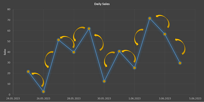
Each observation in the series, except for the initial one, refers back to the preceding observation. This recursive relationship extends to the beginning of the series, giving rise to what are known as long memory models.

Recursive dependency:

Recursive dependency

Order Selection

The order selection is a crucial step in building an AR model as it determines the number of lagged values to include in the model, thereby capturing the relevant dependencies in the time series data.

The primary goal of order selection is to strike a balance between model complexity and model accuracy. A model with a few lagged observations may fail to capture important patterns in the data, leading to underfitting. On the other hand, a model with too many lagged observations may suffer from overfitting, resulting in poor generalization to unseen data.

There are a few commonly used methods to determine the appropriate order (p) for an AR model.

Auto Correlation (ACF — PACF)

The autocorrelation functions are statistical tools to measure and identify the correlation structure in a time series data set.

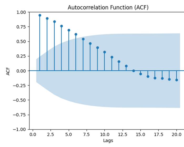
The Autocorrelation Function (ACF) measures the correlation between an observation and its lagged values. It helps in understanding how the observations at different lags are related.

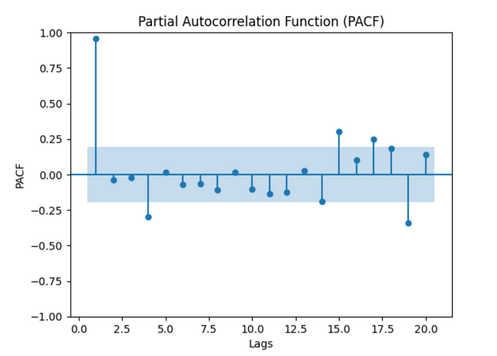
The Partial Autocorrelation Function (PACF) removes the effects of intermediate lags. It measures the direct correlation between two observations.

ACF & PACF:

ACF & PACF.

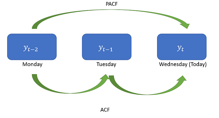
Suppose we observe a positive correlation at a lag of one day. This indicates that there is some correlation between the current day’s price and the previous day’s price. It suggests that the price tends to exhibit a certain degree of persistence from one day to the next.

For example, the reputation of a company is increasing, as its reputation increases, more and more people buy shares of this company. Wednesday’s price is correlated to Tuesday’s which was correlated with Monday's. As the lag increases, the correlation may decrease.

In the case of PACF, there is no influence on the days in between. For example, let’s say an ice cream shop runs a campaign on Mondays and gives free ice cream coupons valid on Wednesdays to anyone who buys ice cream that day. In this case, there will be a direct correlation between the sales on Monday and Wednesday. However, the sales on Tuesday do not affect this situation.

We can use the statsmodels library to plot ACF and PACF in Python.

import numpy as np  
import pandas as pd  
import matplotlib.pyplot as plt  
  
# Generate a random time series data  
np.random.seed(123)  
n_samples = 100  
time = pd.date_range('2023-01-01', periods=n_samples, freq='D')  
data = np.random.normal(0, 1, n_samples).cumsum()  
  
# Create a DataFrame with the time series data  
df = pd.DataFrame({'Time': time, 'Data': data})  
df.set_index('Time', inplace=True)  
  
# Plot the time series data  
plt.figure(figsize=(10, 4))  
plt.plot(df.index, df['Data'])  
plt.xlabel('Time')  
plt.ylabel('Data')  
plt.title('Example Time Series Data')  
plt.show()

Time series data plot:

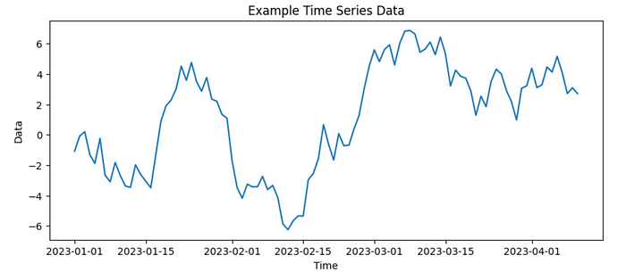
Time series data plot

from statsmodels.graphics.tsaplots import plot_acf  
  
# ACF plot  
plot_acf(df['Data'], lags=20, zero=False)  
plt.xlabel('Lags')  
plt.ylabel('ACF')  
plt.title('Autocorrelation Function (ACF)')

ACF Plot:

ACF Plot

The plot_acf method accepts several parameters:

x is the array of time series data.
lags specifies the lags to calculate the autocorrelation.
alpha is the confidence level, default is 0.05 which corresponds to a 95% confidence level. It means that the confidence intervals in the ACF plot represent the range within which we expect the true population autocorrelation coefficients to fall with 95% probability.

In the ACF plot, the confidence intervals are typically displayed as shaded regions, often in light blue. These intervals indicate the range of values that would be expected for autocorrelations computed from a large number of random samples from a white noise process (where no autocorrelation is present). This means that these intervals represent the range of values that we would expect to see if we were to repeatedly generate random data that does not correlate.

A correlation is considered statistically significant if it falls outside the confidence interval, indicating that it is unlikely to have occurred by chance alone. However, a correlation within the confidence interval does not necessarily imply a lack of correlation, it simply means that the observed correlation is within the range of what we would expect from a white noise process.

use_vlines indicates whether plot vertical lines at each lag to indicate the confidence intervals.
vlines_kwargs is used to define additional parameters for appearance.

from statsmodels.graphics.tsaplots import plot_pacf  
  
plot_pacf(df['Data'], lags=20, zero=False)  
plt.xlabel('Lags')  
plt.ylabel('PACF')  
plt.title('Partial Autocorrelation Function (PACF)')

PACF Plot:

PACF Plot

The plot_pacf accepts the same arguments as parameters, and in addition, we can select which method to use:

“ywm” or “ywmle”: Yule-Walker method without adjustment. It is the default option.
“yw” or “ywadjusted”: Yule-Walker method with sample-size adjustment in the denominator for autocovariance estimation.
“ols”: Ordinary Least Squares regression of the time series on its own lagged values and a constant term.
“ols-inefficient”: OLS regression of the time series on its lagged values using a single common sample to estimate all partial autocorrelation coefficients.
“ols-adjusted”: OLS regression of the time series on its lagged values with a bias adjustment.
“ld” or “ldadjusted”: Levinson-Durbin recursion method with bias correction.
“ldb” or “ldbiased”: Levinson-Durbin recursion method without bias correction.

When evaluating the ACF and PACF plots, firstly look for correlation coefficients that significantly deviate from zero.

Then, notice the decay pattern in the ACF plot. As the lag increases, the correlation values should generally decrease and approach zero. A slow decay suggests a persistent correlation, while a rapid decay indicates a lack of long-term dependence. In the PACF plot, observe if the correlation drops off after a certain lag. A sudden cutoff suggests that the direct relationship exists only up to that lag.

Information Criteria

Information criteria, such as the Akaike Information Criterion (AIC) or Bayesian Information Criterion (BIC), are statistical measures that balance model fit and complexity. These criteria provide a quantitative measure to compare different models with varying orders. The model with the lowest AIC or BIC value is often considered the best-fitting model.

The Akaike Information Criterion (AIC) takes into account how well a model fits the data and how complex the model is. It penalizes complex models to avoid overfitting by including a term that increases with the number of parameters. It seeks to find the model that fits the data well but is as simple as possible. The lower the AIC value, the better the model. It tends to prioritize models with better goodness of fit, even if they are relatively more complex.

The Bayesian Information Criterion (BIC) imposes a stronger penalty on model complexity. It includes a term that grows with the number of parameters in the model, resulting in a more significant penalty for complex models. It strongly penalizes more complexity, favoring simpler models. It is consistent even with a smaller sample size and preferable when the sample size is limited. Again, the lower the BIC value, the better the model.

Now, this time let’s generate more complex data and calculate the AIC and BIC:

import numpy as np  
import matplotlib.pyplot as plt  
from statsmodels.tsa.ar_model import AutoReg  
  
# Generate complex time series data  
np.random.seed(123)  
n = 500  # Number of data points  
epsilon = np.random.normal(size=n)  
data = np.zeros(n)  
  
for i in range(2, n):  
    data[i] = 0.7 * data[i-1] - 0.2 * data[i-2] + epsilon[i]  
  
# Plot the time series data  
plt.figure(figsize=(10, 4))  
plt.plot(data)  
plt.xlabel('Time')  
plt.ylabel('Data')  
plt.title('Time Series Data')  
plt.show()

Time series data:

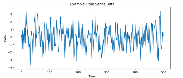
Time series data

# Fit AutoReg models with different orders and compare AIC and BIC  
max_order = 10  
aic_values = []  
bic_values = []  
  
for p in range(1, max_order + 1):  
    model = AutoReg(data, lags=p)  
    result = model.fit()  
    aic_values.append(result.aic)  
    bic_values.append(result.bic)  
  
# Plot AIC and BIC values  
order = range(1, max_order + 1)  
plt.plot(order, aic_values, marker='o', label='AIC')  
plt.plot(order, bic_values, marker='o', label='BIC')  
plt.xlabel('Order (p)')  
plt.ylabel('Information Criterion Value')  
plt.title('Comparison of AIC and BIC')  
plt.legend()  
plt.show()

Comparison of AIC and BIC:

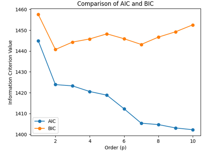
Comparison of AIC and BIC

The AutoReg class is used to fit autoregressive models. It takes several parameters:

endog is the dependent variable.
lags parameter specifies the lag order. It can be an integer representing a single lag value, or a list/array of lag values.
trend determines the trend component included in the model. It can take the following values:

‘c’: adds a constant value to the model equation, allowing for a non-zero mean. It assumes that the trend is a horizontal line.

‘nc’: no constant term. It excludes the constant from the model equation, assuming that the series has a mean of zero. The trend is expected to fluctuate around zero without a systematic upward or downward movement.

‘t’: a linear trend. The model assumes that the trend follows a straight line upward or downward.

‘ct’: combines constant and linear trends.

seasonal indicates whether the model should include a seasonal component.
exog is the exogenous or external variables that we want to include in the model.
hold_back specifies the number of initial observations to exclude from the fitting process.
period is used when seasonal=True and represents the length of the seasonal cycle. It is an integer indicating the number of observations per season.

model.fit() returns an AutoRegResults object and we can get the AIC and BIC from the related attributes.

Since we intentionally generated more complex data, the BIC is expected to favor simpler models more strongly than the AIC. Therefore, the BIC selected a lower-order (simpler) model compared to the AIC, indicating a preference for simplicity while maintaining a reasonable fit to the data.

Ljung-Box Test

The Ljung-Box test is a statistical test used to determine whether there is any significant autocorrelation in a time series.

The test fits an autoregressive model to the data. The residuals of this model capture the unexplained or leftover variation in the data. Then, the Ljung-Box statistic for different lags is calculated. These quantify the amount of residual autocorrelation.

To determine whether the autocorrelation is statistically significant, the Ljung-Box statistic is compared with critical values from a chi-square distribution. These critical values depend on the significance level we choose. If the statistic is higher than the critical value, it suggests the presence of significant autocorrelation, indicating that the model did not capture all the dependencies in the data. On the other hand, if the statistic is lower than the critical value, it implies that the autocorrelation in the residuals is not significant, indicating a good fit for the autoregressive model.

By examining the Ljung-Box test results for different lags, we can determine the appropriate order (p). The lag order with no significant autocorrelation in the residuals is considered suitable for the model.

import numpy as np  
from statsmodels.tsa.ar_model import AutoReg  
from statsmodels.stats.diagnostic import acorr_ljungbox  
  
max_order = 10  
p_values = []  
  
for p in range(1, max_order + 1):  
    model = AutoReg(data, lags=p)  
    result = model.fit()  
    residuals = result.resid  
  
    result = acorr_ljungbox(residuals, lags=[p])  
    p_value = result.iloc[0,1]  
    p_values.append(p_value)  
      
# Find the lag order with non-significant autocorrelation  
threshold = 0.05  
selected_order = np.argmax(np.array(p_values) < threshold) + 1  
print("P Values: ", p_values)  
print("Selected Order (p):", selected_order)  
  
"""  
P Values:  [0.0059441704188493635, 0.8000450392943186, 0.9938379305765744, 0.9928852354721004, 0.8439698152504373, 0.9979352709556297, 0.998574234602306, 0.9999969308975543, 0.9999991895465976, 0.9999997412756536]  
Selected Order (p): 1  
"""

Cross Validation

Cross-validation is another technique for determining the appropriate order (p). Firstly, we divide our time series data into multiple folds or segments. A common choice is to use a rolling window approach, where we slide a fixed-size window across the data.

For each fold, we fit an AR model with a specific lag order (p) using the training portion of the data. Then, we use the fitted model to predict the values for the test portion of the data.

Next, we calculate an evaluation metric (e.g., mean squared error, mean absolute error) and compute the average performance for each fold.

Finally, we choose the lag order (p) that yields the best average performance across the folds.

import numpy as np  
from statsmodels.tsa.ar_model import AutoReg  
from sklearn.metrics import mean_squared_error  
from sklearn.model_selection import TimeSeriesSplit  
  
np.random.seed(123)  
data = np.random.normal(size=100)  
  
max_order = 9  
best_order = None  
best_mse = np.inf  
  
tscv = TimeSeriesSplit(n_splits=5)    
for p in range(1, max_order + 1):  
    mse_scores = []  
      
    for train_index, test_index in tscv.split(data):  
        train_data, test_data = data[train_index], data[test_index]  
          
        model = AutoReg(train_data, lags=p)  
        result = model.fit()  
        predictions = result.predict(start=len(train_data), end=len(train_data) + len(test_data) - 1)  
          
        mse = mean_squared_error(test_data, predictions)  
        mse_scores.append(mse)  
      
    avg_mse = np.mean(mse_scores)  
  
    if avg_mse < best_mse:  
        best_mse = avg_mse  
        best_order = p  
  
print("Best Lag Order (p):", best_order)  
  
"""  
Best Lag Order (p): 3  
"""

Forecasting

In this example, we will consider a dataset of stock prices. Specifically, we will focus on the most recent 40-day period and analyze the stock prices of the company AMD.

We will need these packages.

import datetime  
import numpy as np  
import yfinance as yf  
import matplotlib.pyplot as plt  
from sklearn.metrics import mean_squared_error  
from sklearn.model_selection import TimeSeriesSplit  
from statsmodels.tsa.ar_model import AutoReg  
from statsmodels.graphics.tsaplots import plot_acf, plot_pacf  
from statsmodels.stats.diagnostic import acorr_ljungbox

We can use the yfinance library in Python to access historical stock data from Yahoo Finance.

ticker = "AMD"  
end_date = datetime.datetime.now().date()  
start_date = end_date - datetime.timedelta(days=60)  
data = yf.download(ticker, start=start_date, end=end_date)  
closing_prices = data["Close"]  
print(len(closing_prices))  
  
"""  
[*********************100%***********************]  1 of 1 completed  
42  
"""

plt.figure(figsize=(10, 6))  
plt.plot(closing_prices)  
plt.title("AMD Stock Closing Prices (Last 42 Days)")  
plt.xlabel("Date")  
plt.ylabel("Closing Price")  
plt.xticks(rotation=45)  
plt.grid(True)  
plt.show()

Closing prices:

Closing prices

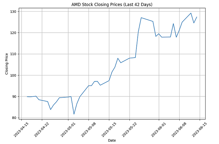
We will split the dataset, designating the most recent record as the test data, while the remaining records will be used for training. Our objective is to build models that can predict the current day’s price. We will evaluate and compare the performance of these models based on their predictions.

n_test = 1  
train_data = closing_prices[:len(closing_prices)-n_test]  
test_data = closing_prices[len(closing_prices)-n_test:]  
print(test_data)  
  
"""  
Date  
2023-06-14    127.330002  
Name: Close, dtype: float64  
"""

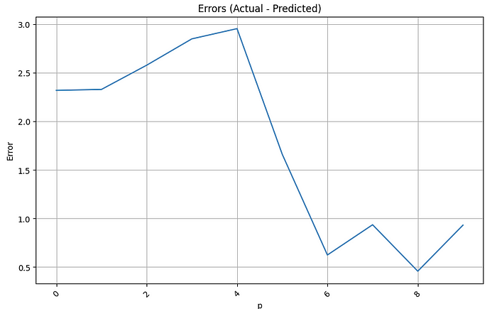
Now, we will proceed to train autoregressive (AR) models with lag orders ranging from 1 to 10. We will use these models to forecast the last price in the dataset and calculate the error for each model.

error_list = []  
for i in range(1,11):  
    model = AutoReg(train_data, lags=i)  
    model_fit = model.fit()  
    predicted_price = float(model_fit.predict(start=len(train_data), end=len(train_data)))  
    actual_price = test_data.iloc[0]  
    error_list.append(abs(actual_price - predicted_price))

plt.figure(figsize=(10, 6))  
plt.plot(error_list)  
plt.title("Errors (Actual - Predicted)")  
plt.xlabel("p")  
plt.ylabel("Error")  
plt.xticks(rotation=45)  
plt.grid(True)  
plt.show()

Errors against p-order values:

Conclusion

We explored the concept of autoregressive (AR) models in time series analysis and forecasting. AR models provide a (starting point) framework for forecasting future values based on past observations.

Order selection (p) is a crucial step in AR modeling, as it determines the number of lagged observations to include in the model. We examined most common techniques for order selection; visual inspection using with ACF and PACF plots, information criteria, Ljung-Box test and cross validation.

AR models offer valuable insights into the dynamics and patterns of time series data, making them invaluable in various domains such as finance, economics, and weather forecasting. By harnessing the power of AR models, we can gain deeper understanding, make accurate predictions, and make informed decisions based on historical patterns and trends.

Time Series Analysis: Mastering the Concepts of Stationarity

Cross-Validation Techniques for Time Series Data

Forecasting Intermittent Demand with Croston’s Method

File Caching in Django

ANOVA Test in Python