Fisher's Linear Discriminant Analysis (LDA) is a dimensionality reduction algorithm that can be used for classification as well. In this blog post, we will learn more about Fisher's LDA and implement it from scratch in Python.
LDA ?
Linear Discriminant Analysis (LDA) is a dimensionality reduction technique. As the name implies dimensionality reduction techniques reduce the number of dimensions (i.e. variables) in a dataset while retaining as much information as possible. For instance, suppose that we plotted the relationship between two variables where each color represent a different class.
WHY ?
The core idea is to learn a set of parameters w ∈ R (d×d′) ,that are used to project the given data x ∈ R (d) to a smaller dimension d′. The figure below (Bishop, 2006) shows an illustration. The original data is in 2 dimensions, d=2 and we want to project it to 1 dimension, d=1.
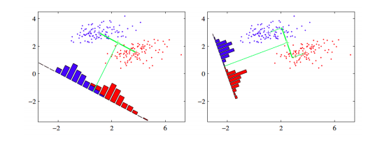
If we project the 2-D data points onto a line (1-D), out of all such lines, our goal is to find the one which maximizes the distance between the means of the 2 classes, after projection. If we could do that, we could achieve a good separation between the classes in 1-D. This is illustrated in the figure on the left and can be captured in the idea of maximizing the “between class covariance”. However, as we can see that this causes a lot of overlap between the projected classes. We want to minimize this overlap as well. To handle this, Fisher's LDA tries to minimize the “within-class covariance” of each class. Minimizing this covariance leads us to the projection in the figure on the right hand side, which has minimal overlap. Formalizing this, we can represent the objective as follows.
Minimize this expression = Objective of Fischer LDA
Where Sb ∈ R (d×d)and Sw ∈ R (d×d)are the between-class and within-class covariance matrices, respectively. They are calculated as:
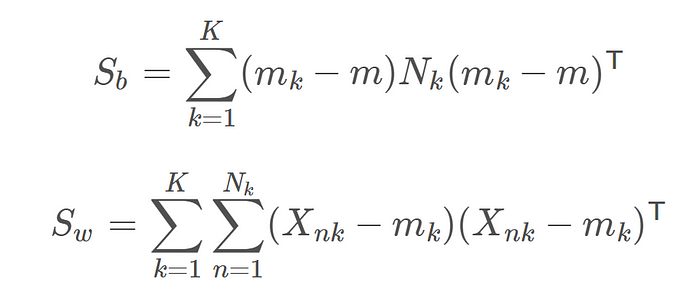
Calculation of Sb and Sw
Where Xnk is the nth data example in the kth class, Nk is the number of examples in class k, m is the overall mean of the entire data and mk is the mean of the kth class. Now using Lagrangian dual and the KKT conditions, the problem of maximizing J can be transformed into the solution:
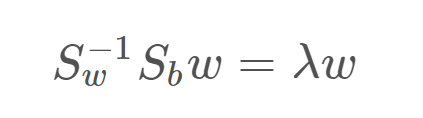
Which is an eigenvalue problem for the matrix inv(Sw).Sb . Thus our final solution for w will be the eigenvectors of the above equation, corresponding to the largest eigenvalues. For reduction to d′ dimensions, we take the d′ largest eigenvalues as they will contain the most information. Also, note that if we have K classes, the maximum value of d′ can be K−1. That is, we cannot project K class data to a dimension greater than K−1. (Of course, d′ cannot be greater than the original data dimension d). This is because of the following reason.
Note that the between-class scatter matrix, Sb was a sum of K matrices, each of which is of rank 1, being an outer product of two vectors. Also, because the overall mean and the individual class means are related, only (K−1) of these K matrices are independent. Thus Sb has a maximum rank of K−1 and hence there are only K−1 non-zero eigenvalues. Thus we are unable to project the data to more than K−1 dimensions.
HOW ?
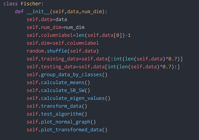
In short , following are the key steps to be followed:
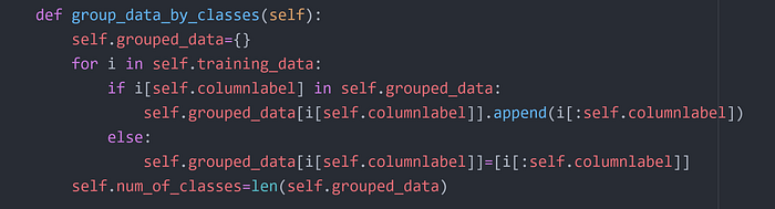
- Group the training data into it's respective classes . i.e Form a dictionary and save data grouped by classes it belongs to.
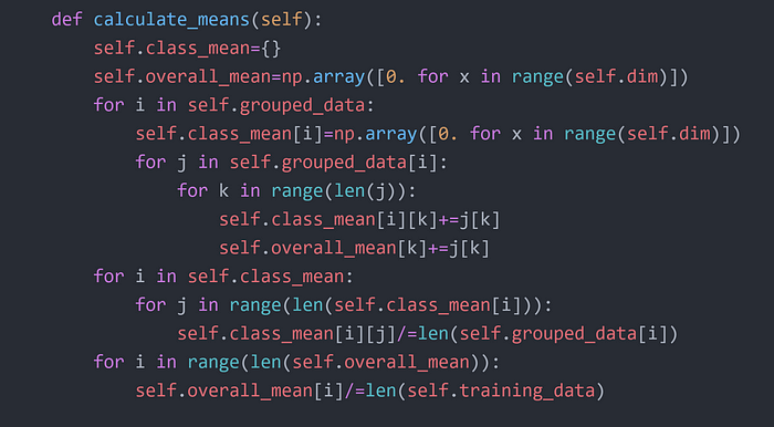
- Calculate mean vector of given training data of K-dimensions excluding the target class and also calculate class-wise mean vector for the given training data.
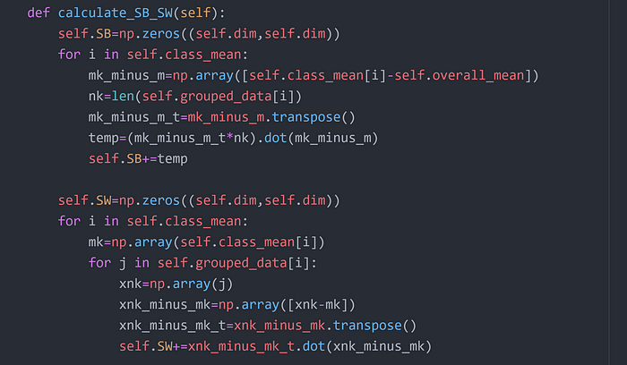
- Calculate SB and SW matrices needed to maximize the difference between means of given classes and minimize the variance of given classes.
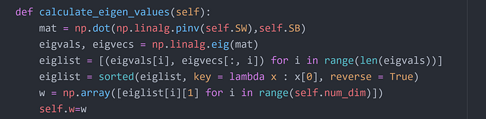
- After that calculate the matrix M , where M = (inv(SW)).(SB)
- Calculate eigen values of M and get eigen vector pairs for first n (needed ) dimensions.
- This eigen vectors give us the value of 'w' used to transform points to needed number of dimensions.
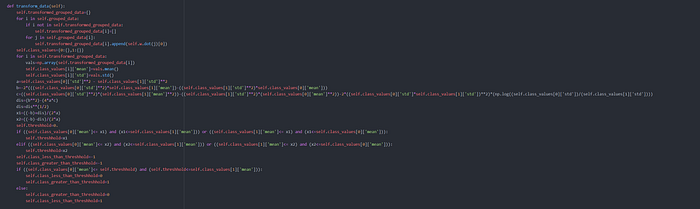
- After applying the transformation to every point i.e. Transformed_Point = w.dot(given_point) , we calculate the threshhold value by which we will classify points into positive and negative class.
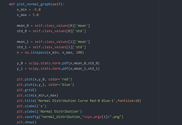
- To calculate Threshhold use Gaussian Normal Distribution.
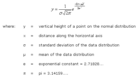
Normal Equation
- After calculating Normal Equation of both classes , we get threshhold value and then classify points by threshhold.
Here is the Python Implementation step wise :
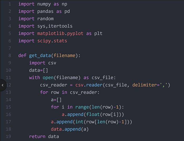
Step 1
Step 2
Step 3
Step 4
Step 5
Step 6
Step 7
Step 8
Step 9
Step 10
Step 11
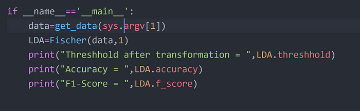
After coding this to run the fischer program in python you need to run following command :
python fischer.py dataset_name.csv
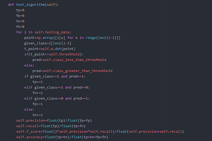
This will generate all plots and give accuracy and f1-score for the classification.
Experiments :
- Dataset is a1_d1.csv that can be downloaded from here.
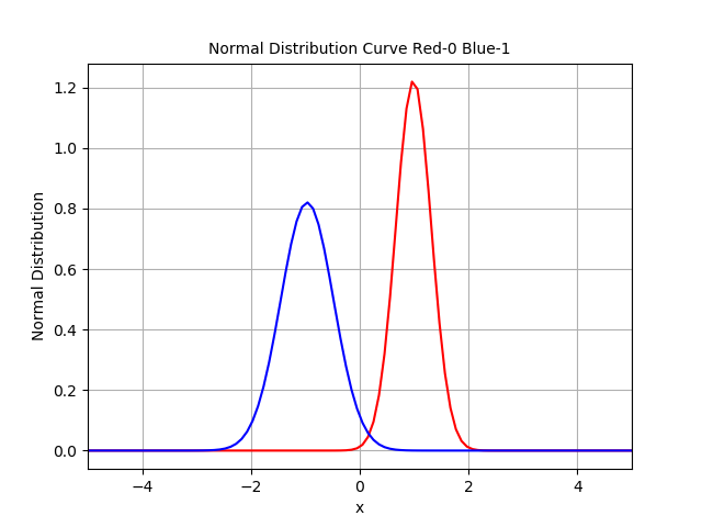
Normal Distribution Curve after transformation. Intersection Point = Threshhold
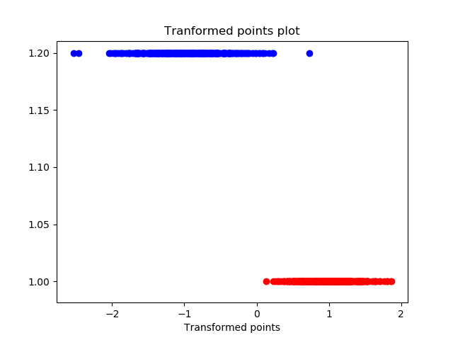
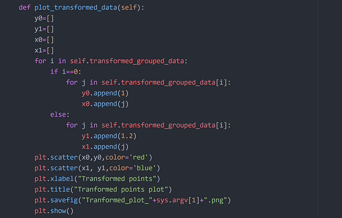
Transformed points
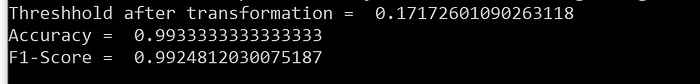
Results
References :
- Bishop, C. M. (2006). Pattern recognition. Machine Learning, 128.
Comments
Loading comments…