Gaussian Distribution In Machine Learning

Introduction

The Gaussian distribution is the healthy-studied probability distribution. It is for nonstop-valued random variables. It is as well stated as the normal distribution. Its position makes from the fact that it has many computationally suitable properties.

The Gaussian distribution is the backbone of Machine Learning. Every data scientist needs to know during working with linear models. It was learnt by Carl Friedrich Gauss.

Description

There are several parts of machine learning that takes advantage from using a Gaussian distribution. Those areas are including;

• Gaussian processes
• Variational inference
• Reinforcement learning

It is similarly broadly used in other application areas such as

• Signal processing such as Kalman filter
• Control, for example linear quadratic regulator
• Statistics, as hypothesis testing

Practical uses

• Designing Standardized Tests: These are designed as a result that test-taker scores fall within a Gaussian distribution.
• Statistical Tests: There may be several statistical Tests are derived from a Gaussian distribution.
• Quantum Mechanics: The Gaussian distribution may be used to define the ground state of a quantum harmonic oscillator.

Importance of Gaussian Distribution

• It is ever-present as a dataset with finite variance turns into Gaussian as long as dataset with free feature-probabilities is permitted to raise in size.
• It is the most significant probability distribution in statistics as it turns many natural phenomena such as age, height, test-scores, IQ scores, and sum of the rolls of two cubes and so on.
• Datasets with Gaussian distributions creates valid to a diversity of methods that decrease under parametric statistics.
• The approaches for example propagation of uncertainty and least squares parameter right are related only to datasets with normal or normal-like distributions.
• Reviews and conclusions resulting from such analysis are intuitive. That also easy to explain to audiences with basic knowledge of statistics.

Parameters of Gaussian Distribution

The mean and standard deviation are two main parameters of a Gaussian Distribution. We may decide the shape and probabilities of the distribution with respect to our problem statement by the help of these parameters. The shape of the distribution changes when the parameter value changes.

Mean

• Scientists used the mean or average value as a measure of dominant trend.
• It may be used to define the distribution of variables that are measured as ratios or intervals.
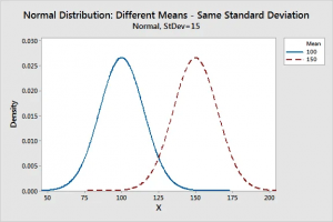
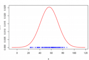
• The mean decides the site of the peak. The many of the data points are gathered around the mean in a normal distribution graph.
• By changing the value of the mean we can move the curve of Gaussian Distribution moreover to the left or right along the X-axis.

Standard Deviation

• It acts how the data points are circulated comparative to the mean.
• It fixes how distant the data points are missing from the mean.
• It characterizes the distance between the mean and the data points.
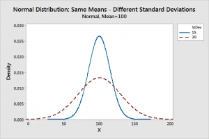
• It describes the width of the graph. Consequently, varying the value of standard deviation make tighter or enlarges the width of the distribution along the x-axis.
• A lesser standard deviation with respect to the mean results in a steep curve and a greater standard deviation marks in a flatter curve.

• When a single variable x, the Gaussian distribution may be written in the form:

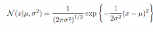
• where μ is the mean and σ2 is the variance
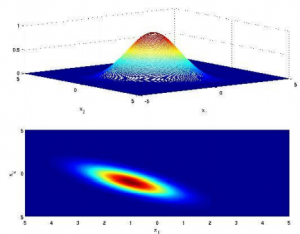
• For a D-dimensional vector x, the multivariate Gaussian distribution can be written in the form:

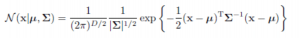
• where μ is a D-dimensional mean vector
• Σ is a D xD covariance matrix
• |Σ| denotes the determinant of Σ

Plotting Gaussian Distribution in Python

In Python, we have libraries for example Numpy, scipy, and matplotlib. These are very supportive for us to plot an ideal normal curve.

import numpy as np
import scipy as sp
from scipy import stats
import matplotlib.pyplot as plt
## generate the data and plot it for an ideal normal curve
## x-axis for the plot
x_data = np.arange(-5, 5, 0.001)
## y-axis as the gaussian
y_data = stats.norm.pdf(x_axis, 0, 1)
## plot data
plt.plot(x_data, y_data)plt.show()

Output

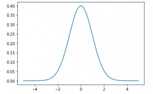
• The points on the x-axis are the observations.
• The points on y-axis is the probability of each observation.
• We created commonly spaced observations in the range (-5, 5) using np.arange().
• Then we ran it through the norm.pdf() function with a mean of 0.0.
• The standard deviation is 1 that returned the probability of that observation.
• Remarks around 0 are the most common and the ones around -5.0 and 5.0 are rare.
• The technical word for the pdf() function is the probability density function.

For more details visit: https://www.technologiesinindustry4.com/2021/09/gaussian-distribution-in-machine-learning.html