Convolutional Autoencoders (CAE) with Tensorflow

Autoencoders has been in the deep learning literature for a long time now, most popular for data compression tasks. With their easy structure and not so complicated underlying mathematics, they became one of the first choices when it comes to dimensionality reduction in simple data. However, using basic fully connected layers fail to capture the patterns in pixel-data since they do not hold the neighboring information. For a good capturing of the image data in latent variables, convolutional layers are usually used in autoencoders.

For the previous post on Autoncoders, please visit:

AutoEncoders with TensorFlow

Introduction

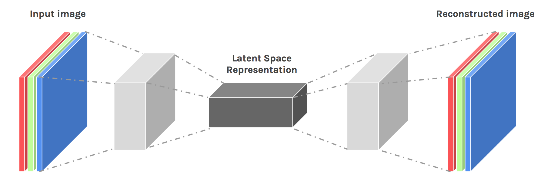
Autoencoders are unsupervised neural network models that summarize the general properties of data in fewer parameters while learning how to reconstruct it after compression[1]. In order to extract the textural features of images, convolutional neural networks provide a better architecture. Moreover, CAEs can be stacked in such a way that each CAE takes the latent representation of the previous CAE for higher-level representations[2]. Nevertheless, in this article, a simple CAE will be implemented having 3 convolutional layers and 3 subsampling layers in between.

The tricky part of CAEs is at the decoder side of the model. During encoding, the image sizes get shrunk by subsampling with either average pooling or max-pooling. Both operations result in information loss which is hard to re-obtain while decoding.

There are both straightforward and smarter ways to perform this upsampling. The most basic method is populating the same image pixel while increasing the image size by the upsampling rate.

Some models hold the location of the maximum value during encoding and then only give activation to that location while surpassing the others.

It is also possible to do the mapping from smaller size to larger size with learned weights. However, in this implementation, we will continue with the basic upsampling procedure. The overall architecture mostly resembles the autoencoder that is implemented in the previous post, except 2 fully connected layers are replaced by 3 convolutional layers.

A Simple Convolutional Autoencoder with TensorFlow

A CAE will be implemented including convolutions and pooling in the encoder, and deconvolution in the decoder. The model is tested on the Stanford Dogs Dataset[6]. For a simple implementation, Keras API on TensorFlow backend is preferred with Google Colab GPU services.

First, needed libraries are imported.

import tensorflow as tf
import matplotlib.pyplot as plt
from tensorflow.keras import datasets, layers, models, losses, Model
from random import randint
import numpy as np

The Data

The data is directly loaded into the Google Colab session from Kaggle. You can follow the steps nicely explained here to load the data. Please first go to Kaggle and sign in to your account. From the top-right of the page click on the icon and go to Account. Then click “Expire API Tokens” and “Create New API Token”, respectively. You will download a file named “kaggle.json”.

! pip install -q kaggle

from google.colab import files
files.upload()

! mkdir ~/.kaggle

! cp kaggle.json ~/.kaggle/

! chmod 600 ~/.kaggle/kaggle.json

! kaggle datasets download -d miljan/stanford-dogs-dataset-traintest

As you run the code above you will

1. Install the Kaggle API

2. Upload the “.json” file

3. Create a directory called “.kaggle” and copy the downloaded file there

4. Make the file executable

5. Finally, download the dataset.

The data is unzipped in the path, “/content/”.

import os
os.chdir('/content')

!unzip -q 'stanford-dogs-dataset-traintest.zip'

Then, the files are stored in variables for ease of use. The file names for the train and test images are stored in a list using os.walk. Then the images are read into a tensor.

import numpy as np
import matplotlib.pyplot as plt

files=[]

for root, _, filenames in os.walk('/content/cropped/train'):
  for filename in filenames:
    files.append(os.path.join(root,filename))

x_train = []
for f in files:
  x_train.append(plt.imread(f))

files=[]

for root, _, filenames in os.walk('/content/cropped/test'):
  for filename in filenames:
    files.append(os.path.join(root,filename))

x_test = []
for f in files:
  x_test.append(plt.imread(f))

x_train = np.asarray(x_train)
x_test = np.asarray(x_test)

A sample from the dataset is as follows:

The Encoder

The encoder model consists of three convolution layers having features maps of sizes 32, 64, and 128 each followed by a max-pooling subsampling. The 3x3 kernels and ReLU activations are also used.

encoder = models.Sequential()

encoder.add(layers.Conv2D(32, 3, strides=1, padding='same', activation='relu', input_shape=x_train.shape[1:]))
encoder.add(layers.MaxPooling2D(2, strides=2))

encoder.add(layers.Conv2D(64, 3, strides=1, padding='same', activation='relu'))
encoder.add(layers.MaxPooling2D(2, strides=2))

encoder.add(layers.Conv2D(128, 3, strides=1, padding='same', activation='relu'))
encoder.add(layers.MaxPooling2D(2, strides=2))

encoder.summary()

Model: "sequential_9" _________________________________________________________________ Layer (type)                 Output Shape              Param #    ================================================================= conv2d_27 (Conv2D)           (None, 224, 224, 32)      896        _________________________________________________________________ max_pooling2d_24 (MaxPooling (None, 112, 112, 32)      0          _________________________________________________________________ conv2d_28 (Conv2D)           (None, 112, 112, 64)      18496      _________________________________________________________________ max_pooling2d_25 (MaxPooling (None, 56, 56, 64)        0          _________________________________________________________________ conv2d_29 (Conv2D)           (None, 56, 56, 128)       73856      _________________________________________________________________ max_pooling2d_26 (MaxPooling (None, 28, 28, 128)       0          ================================================================= Total params: 93,248 Trainable params: 93,248 Non-trainable params: 0

The Decoder

The decoder takes the tensor having the sizes of (batch size, 28, 28, 128) from the encoder and passes it through convolutional layers having the feature map size of 128, 16, and 3. The resulting tensor has a channel size of 3 representing the RGB. Simple upsampling is performed as described earlier.

decoder = models.Sequential()

decoder.add(layers.Conv2D(128, 3, strides=1, padding='same', activation='relu', input_shape=encoder.output.shape[1:]))
decoder.add(layers.UpSampling2D(2))

decoder.add(layers.Conv2D(16, 3, strides=1, padding='same', activation='relu'))
decoder.add(layers.UpSampling2D(2))

decoder.add(layers.Conv2D(3, 3, strides=1, padding='same', activation='relu'))
decoder.add(layers.UpSampling2D(2))

decoder.summary()

Model: "sequential_10" _________________________________________________________________ Layer (type)                 Output Shape              Param #    ================================================================= conv2d_30 (Conv2D)           (None, 28, 28, 128)       147584     _________________________________________________________________ up_sampling2d_3 (UpSampling2 (None, 56, 56, 128)       0          _________________________________________________________________ conv2d_31 (Conv2D)           (None, 56, 56, 16)        18448      _________________________________________________________________ up_sampling2d_4 (UpSampling2 (None, 112, 112, 16)      0          _________________________________________________________________ conv2d_32 (Conv2D)           (None, 112, 112, 3)       435        _________________________________________________________________ up_sampling2d_5 (UpSampling2 (None, 224, 224, 3)       0          ================================================================= Total params: 166,467 Trainable params: 166,467 Non-trainable params: 0

The Autoencoder

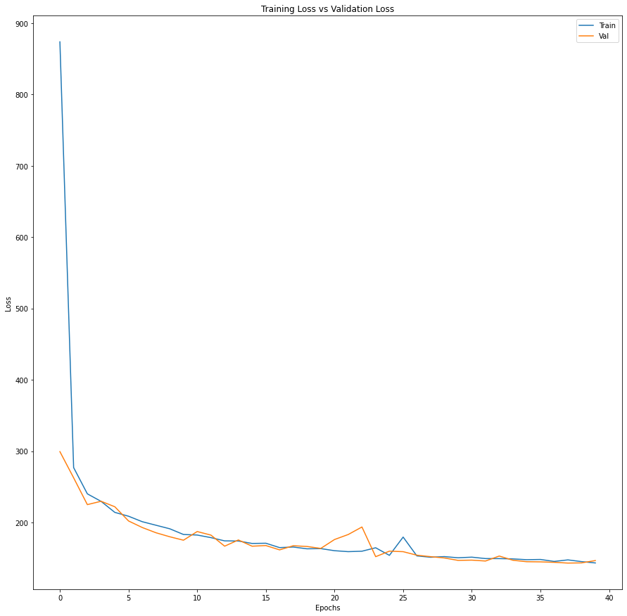
CAE is constructed by setting the computation graph. Model is compiled and trained with *Adam *optimizer, mean squared error loss, and a batch size of 64 for 40 epochs.

conv_autoencoder = Model(inputs=encoder.input, outputs=decoder(encoder.outputs))

conv_autoencoder.compile(optimizer='adam', loss=losses.mean_squared_error)

history = conv_autoencoder.fit(x_train, x_train, batch_size=64, epochs=40, validation_data=(x_test, x_test))

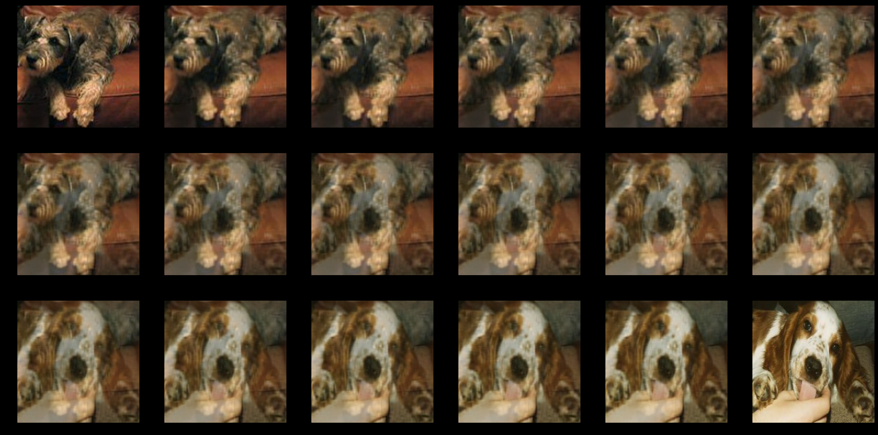
A similar approach to what has been done in the previous post for qualitative analysis is followed here as well. Taking two random images and encoding them into latent space, then interpolating 16 more latent vectors between the original vectors, and finally decoding them yielded the results below. We can observe the gradual shift from one dog breed to another one.

Final Remark: Please do not forget to leave some food and water outside your apartment for the street animals.

convolutional_autoencoder_tensorflow.ipynb

Conclusion

As compared to the Autoencoders with fully connected layers, Convolutional Autoencoders does a better job to encapsulate the underlying patterns in the pixel data. In this article, a more challenging dataset is used with larger image sizes and RGB channels. Still, CAE performs at least as well as a standard Autoencoder through the qualitative analysis.

Hope you enjoyed it. See you in the following Autoencoder applications.

Best wishes…

mrgrhn

References

1. Gallinari, P., LeCun, Y., Thiria, S., & Fogelman-Soulie, F. (1987). “Memoires associatives distribuees”. Proceedings of COGNITIVA 87. Paris, La Villette.

2. Masci, Jonathan & Meier, Ueli & Ciresan, Dan & Schmidhuber, Jürgen. (2011). “Stacked Convolutional Auto-Encoders for Hierarchical Feature Extraction”. 52–59. 10.1007/978–3–642–21735–7_7.

3. Aljaafari, Nura. (2018). “Ichthyoplankton Classification Tool using Generative Adversarial Networks and Transfer Learning”.

4. https://zhuanlan.zhihu.com/p/67510665

5. https://www.programmersought.com/article/2908798542/

6. Khosla, A., Jayadevaprakash, N., Yao, B., & Fei-Fei, L. (2012). “Novel Dataset for Fine-Grained Image Categorization: Stanford Dogs”.

7. http://vision.stanford.edu/aditya86/StanfordDogs/