This is my first post and this post is for an absolute beginner. If you are stuck somewhere in this tutorial then don't worry about that. This post is just for you to make you familiar with the machine learning process, In the upcoming series of posts, we will discuss in-depth about the concepts.
In this post, you will make your first machine learning project (step-by-step) in Python.
Overview of what we are going to cover:
- Setting up the Environment.
- Loading the dataset.
- Summarizing the data.
- Data visualization.
- Model Building- part 1.
- Model Building- part 2.
Photo by Andy Kelly on Unsplash
This post is 1 day of the “10 days of machine learning project” post series. **_1–3 days** — Beginners project tutorials 4–6 days — Intermediate project tutorials **7–10 days** — Advanced project tutorials
Machine Learning in Python: Step-By-Step Tutorial (start here)
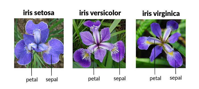
It is called a hello world program of machine learning and it's a classification problem where we will predict the flower class based on its petal length, petal width, sepal length, and sepal width.
1. Setting up the Environment:
In this tutorial we are going to use Google Colab, hope you guys are familiar with Google Colab.
Google Colab provides a jupyter notebook to run your code without installing any software or libraries in your local machine.
1.1 Search ‘google colab' in your browser or CLICK HERE to go to the colab website:
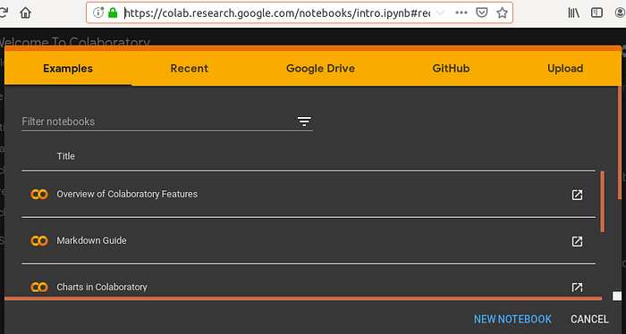
Create a new Notebook written in blue color
1.2. Click on New Notebook , to create a new notebook in google colab where
we will write our code:

Press Shift+Enter to run the cell in notebook
2. Loading the dataset:
First of all we will import some libraries for analysis and model building:
# IMPORTING LIBRARIES
import numpy as np
import pandas as pd
import seaborn as sns
sns.set_palette('husl')
import matplotlib.pyplot as plt
%matplotlib inline
from sklearn.model_selection import train_test_split
from sklearn.model_selection import cross_val_score
from sklearn.model_selection import StratifiedKFold
from sklearn.metrics import classification_report
from sklearn.metrics import accuracy_score
from sklearn.linear_model import LogisticRegression
from sklearn.tree import DecisionTreeClassifier
from sklearn.neighbors import KNeighborsClassifier
from sklearn.discriminant_analysis import LinearDiscriminantAnalysis
from sklearn.naive_bayes import GaussianNB
from sklearn.svm import SVC
Loading Iris data
This is the URL of the dataset, where the data of the iris flower is stored:
https://raw.githubusercontent.com/jbrownlee/Datasets/master/iris.csv
We will assign this link to "url" variable:
url = 'https://raw.githubusercontent.com/jbrownlee/Datasets/master/iris.csv'
Creating the list of column name:
col_name = ['sepal-lenght','sepal-width','petal-lenght','petal-width','class']
Pandas read_csv() is used for reading the csv file:
dataset = pd.read_csv(url, names = col_name)
3. Summarize the Dataset
Let's check the shape of the data on which we have to work on:
dataset.shape
Output:
(150, 5)
This shows that we have 150 rows and 5 columns.
Now displaying the first 5 records of our dataset:
dataset.head()
Output:
sepal-lenght sepal-width  petal-lenght petal-width       class
        5.1       3.5       1.4         0.2            Iris-setosa
        4.9       3.0       1.4         0.2            Iris-setosa
        4.7       3.2       1.3         0.2            Iris-setosa
        4.6       3.1       1.5         0.2            Iris-setosa
        5.0       3.6       1.4         0.2            Iris-setosa
Pandas info() method prints information about a DataFrame including the index dtype and columns, non-null values and memory usage:
dataset.info()
Output:
<class 'pandas.core.frame.DataFrame'>
RangeIndex: 150 entries, 0 to 149
Data columns (total 5 columns):
 #   Column        Non-Null Count  Dtype
---  ------        --------------  -----
 0   sepal-lenght  150 non-null    float64
 1   sepal-width   150 non-null    float64
 2   petal-lenght  150 non-null    float64
 3   petal-width   150 non-null    float64
 4   class         150 non-null    object
dtypes: float64(4), object(1)
memory usage: 6.0+ KB
Pandas describe() is used to view some basic statistical details like percentile, mean, std etc. of a data frame or a series of numeric values:
dataset.describe()
Output:
count  150.000000     150.000000     150.000000     150.000000
mean     5.843333       3.054000       3.758667       1.198667
std       0.828066       0.433594       1.764420       0.763161
min       4.300000       2.000000       1.000000       0.100000
25%       5.100000       2.800000       1.600000       0.300000
50%       5.800000       3.000000       4.350000       1.300000
75%       6.400000       3.300000       5.100000       1.800000
max       7.900000       4.400000       6.900000       2.500000
We can see that numerical values are in range of 0 to 8.
Now let's check the number of rows that belongs to each class:
dataset['class'].value_counts()
Output:
Iris-virginica     50
Iris-setosa        50
Iris-versicolor    50
Name: class, dtype: int64
We can see that each class of flowers has 50 rows.
4. Data Visualization
Violin plot
Plotting the violin plot to check the comparison of a variable distribution:
sns.violinplot(y='class', x='sepal-lenght', data=dataset, inner='quartile')
plt.show()
sns.violinplot(y='class', x='sepal-width', data=dataset, inner='quartile')
plt.show()
sns.violinplot(y='class', x='petal-lenght', data=dataset, inner='quartile')
plt.show()
sns.violinplot(y='class', x='petal-width', data=dataset, inner='quartile')
plt.show()
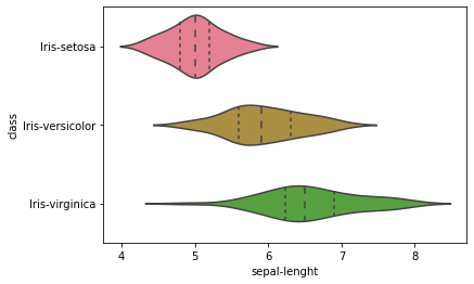
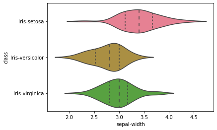
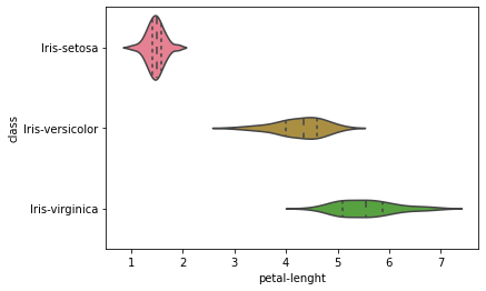
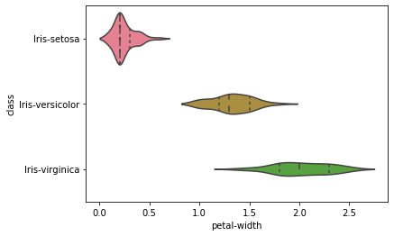
The above-plotted violin plot says that Iris-Setosa class is having a smaller petal length and petal width compared to other class.
**Pair plot
**Plotting multiple pairwise bivariate distributions in a dataset using pairplot:
sns.pairplot(dataset, hue='class', markers='+')
plt.show()
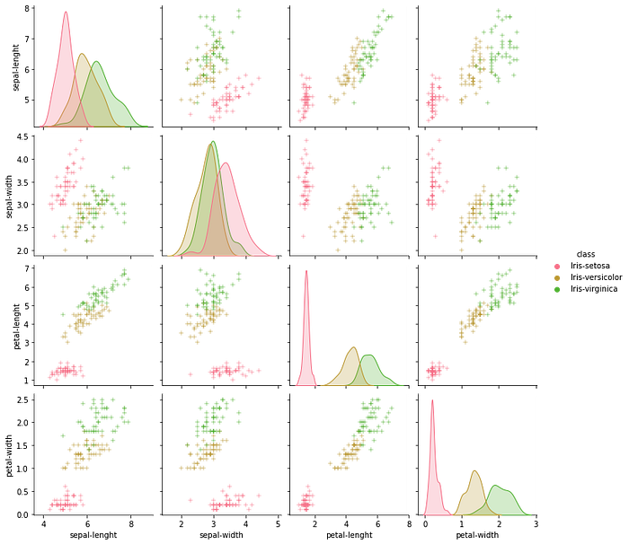
From the above, we can see that Iris-Setosa is separated from both other species in all the features.
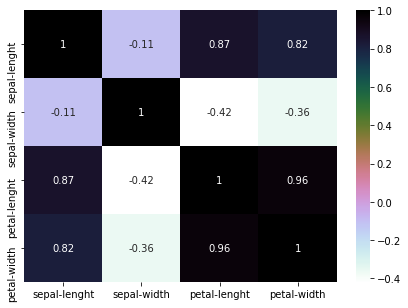
**Heatmap
**Plotting the heatmap to check the correlation.
dataset.corr() is used to find the pairwise correlation of all columns in the dataframe.
plt.figure(figsize=(7,5))
sns.heatmap(dataset.corr(), annot=True, cmap='cubehelix_r')
plt.show()
5. Model Building- part 1
**5.1 Splitting the dataset
**X is having all the dependent variables.
Y is having an independent variable (here in this case ‘class' is an independent variable).
X = dataset.drop(['class'], axis=1)
y = dataset['class']
print(f'X shape: {X.shape} | y shape: {y.shape} ')
Output:
X shape: (150, 4) | y shape: (150,)
Here, we can see from the output that the X has 150 rows and 4 columns whereas Y has 150 rows and only one column.
**5.2 Train Test split
**Splitting our dataset into train and test using train_test_split(), what we are doing here is taking 80% of data to train our model, and 20% that we will hold back as a validation dataset:
X_train, X_test, y_train, y_test = train_test_split(X, y, test_size=0.20, random_state=1)
**5.3 Model Creation
**We don't know which algorithms would be best for this problem.
Let's check each algorithm in loop and print its accuracy, so that we can select our best algorithm.
Let's test 6 different algorithms:
- Logistic Regression (LR)
- Linear Discriminant Analysis (LDA)
- K-Nearest Neighbors (KNN).
- Classification and Regression Trees (CART).
- Gaussian Naive Bayes (NB).
- Support Vector Machines (SVM).
I know at this point you are thinking that it is so complicated to understand the below code, but don't worry about it. In the next step, I will explain how to train and check the accuracy of the model manually.
models = []
models.append(('LR', LogisticRegression()))
models.append(('LDA', LinearDiscriminantAnalysis()))
models.append(('KNN', KNeighborsClassifier()))
models.append(('CART', DecisionTreeClassifier()))
models.append(('NB', GaussianNB()))
models.append(('SVC', SVC(gamma='auto')))
# evaluate each model in turn
results = []
model_names = []
for name, model in models:
kfold = StratifiedKFold(n_splits=10, random_state=1, shuffle=True)
cv_results = cross_val_score(model, X_train, y_train, cv=kfold, scoring='accuracy')
results.append(cv_results)
model_names.append(name)
print('%s: %f (%f)' % (name, cv_results.mean(), cv_results.std()))
Output:
LR: 0.966667 (0.040825)
LDA: 0.975000 (0.038188)
KNN: 0.958333 (0.041667)
CART: 0.950000 (0.055277)
NB: 0.950000 (0.055277)
SVC: 0.983333 (0.033333)
Support Vector Classifier (SVC) is performing better than other algorithms.
Let's train SVC model on our training set and predict on test set in the next step.
**6. Model Building- part 2
**6.1. We are defining our SVC model and passing gamma as auto. If you wanted to know more about parameter visit this link.
6.2. After that fitting/training the model on X_train and Y_train using .fit() method.
6.3. Then we are predicting on X_test using .predict() method.
model = SVC(gamma='auto')
model.fit(X_train, y_train)
prediction = model.predict(X_test)
6.4. Now checking the accuracy of our model using
accuracy_score(y_test, prediction)
y_test: actual values of X_test
prediction: predicted values of X_test (refer to point 3).
6.5. Printing out the classification report using
classification_report(y_test, prediction).
print(f'Test Accuracy: {accuracy_score(y_test, prediction)}')
print(f'Classification Report: \n {classification_report(y_test, prediction)}')
Output:
Accuracy: 0.9666666666666667
Classification Report:
                  precision    recall  f1-score   support
Iris-setosa           1.00      1.00      1.00        11
Iris-versicolor       1.00      0.92      0.96        13
 Iris-virginica       0.86      1.00      0.92         6

       accuracy                           0.97        30
      macro avg       0.95      0.97      0.96        30
   weighted avg       0.97      0.97      0.97        30
You can repeat this process with other algorithms to check the accuracy of model manually.
Machine learning project tutorial for beginners
Congratulations! You just created you first machine learning project.
What to do next ?
As was mentioned earlier in this post that this is the 1 Day post of my 10 days of machine learning post series. I will post beginner level to advanced level project tutorials, So follow this blog for more upcoming tutorials.
If you have any doubt regarding this tutorial please feel free to comment down your questions, I'm going to answer each and every comment you post in my blog.
Connect with me on LinkedIn: Md Injemamul Irshad
Comments
Loading comments…