Have you ever thought while working with gradient descent that there should be some other optimization algorithms to try out? If you have then the good news is we have some global optimization algorithms in the form of genetic and swarm algorithms widely known as biologically inspired algorithms.
Inspired by Charles Darwin’s theory of natural evolution, genetic algorithms support natural selection, in which the fittest individuals are chosen for reproduction in order to generate the following generation’s progeny. This algorithm is an evolutionary algorithm that uses natural selection with a binary representation and simple operators based on genetic recombination and genetic mutations to execute an optimization procedure influenced by the biological theory of evolution.
Knapsack problem:
In this article, we will implement a genetic algorithm to solve the knapsack problem. The knapsack problem is a combinatorial optimization problem in which you must determine the number of each item to include in a collection so that the total weight is less than or equal to a given limit and the total value is as large as possible given a set of items, each with a weight and a value.
**Natural Selection Ideology:
**The selection of the fittest individuals from a population begins the natural selection process. They generate offspring who inherit the parents’ qualities and are passed down to the next generation. If parents are physically active, their children will be fitter than they are and have a better chance of surviving. This procedure will continue to iterate until a generation of the fittest individuals is discovered.
The genetic algorithm cycle is divided into the following components which are the building blocks of this algorithm:
-
Fitness Function
-
Chromosome Initialization
-
Initialize the population
-
Fitness Evaluation
-
Roulette Selection
-
Crossover
-
Mutation
Cycle of Genetic Algorithm:
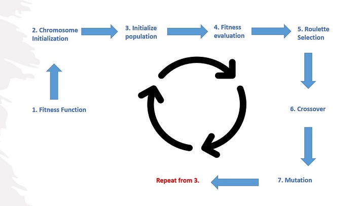
This cycle from 3 will be repeated until we have an optimized solution.
We will implement each one and then put it all together to apply it to the knapsack problem but before implementing the Genetic algorithm let's understand what the parameters of the Genetic Algorithm are.
Parameters of Genetic Algorithm:
- chromosome size — dimension of the chromosome vector. In our case, we have 64 items so the chromosome size is equal to 64
- population size — number of individuals in the population
- parent count — number of parents that are selected from the population on the base of the roulette selection. The parent count must be less than the population size.
- probability of ones in a new chromosome — probability which is used for initial population generation. It is the probability of one in the initial chromosome. High values may lead to the generation of many individuals with fitness equal to zero. This parameter is specific to our method of generation of the initial chromosome. This parameter is meaningless if your choice is any other method.
- probability of crossover — the probability of crossover i.e., if the child inherits the gene of both parents or 1.
- probability of mutation — the probability of mutation. I recommend starting at the value of 1/chromosome size and increasing later as you see the change
Implementation
- Fitness Function:
The fitness function determines an individual’s level of fitness (the ability of an individual to compete with other individuals). It assigns everyone a fitness score. The fitness score determines the likelihood of an individual being chosen for reproduction
Let w is the weight vector, c is the cost vector, g is a chromosome and L is the weight limit, we define the fitness function as:
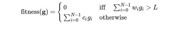
Now let’s implement the function:
#fitness function for each chromosome

def fitness(w, c, L, g): #weight, cost, weight_limit, chromosome
  score = 0
  score1 = 0
  for i in range(len(w)):
    score = score + np.sum(w[i]*g[i])
  if score > L:
      f = 0
  else:
    for i in range(len(w)):
      score1 = score1 + np.sum(c[i]*g[i])
    f = score1
  return score1, score #fitness
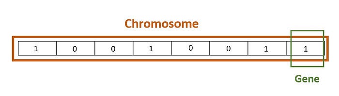
2. Chromosome Initialization:
After defining the fitness function, we will initialize chromosomes for each individual in our population. A set of factors (0/1) known as Genes characterizes an individual. To build a Chromosome, genes are connected in a string.
Chromosome also known as individual:
Let p is the initialization probability for 1 in a new chromosome, ψ is a random value with the unique distribution in the range of <0,1> and g be a new chromosome then:
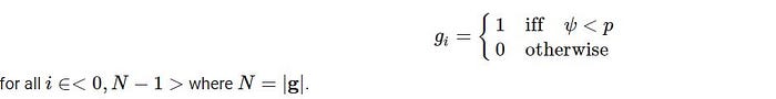
To ensure that the probability should be sufficiently low to generate a valid solution with non-zero fitness. Check the validity of the solution after chromosome creation and recreate it if the total weight of the knapsack is above the weight limit L. More formally for a valid solution.

Where w is the weight vector. This is recommended, but the not mandatory way how to initialize a new chromosome. Be aware that producing non-valid solutions with zero fitness at the start may disturb the algorithm. Let’s initialize the chromosomes as:
#generating chromosome with probability of 1's
import random
def generate_chromosome(N, w, L, p): #N choromosome_size, weight, #limit, probability
  score = 0
  g = np.zeros(N) #verify if vector is 64 or 65
  for i in range(len(g)):
    prob = random.uniform(0, 1)
    if prob < p:
      g[i] = 1
    else:
      g[i] = 0
  for c in range(N):
    score = score + np.sum(w[c]*g[c])
  if score <= L:
    pass
  return g
3. Initialize population:
Now we will initialize our population, The population is represented by a NumPy matrix. Rows of the matrix correspond to individuals, columns correspond to genes in the chromosome. Our matrix has 64 columns because we have 64 items. This can change depending on your problem.
We will initialize the population using the generate_chromosome() function as:
#initializing population by generating chromosome
def initialize_population(population_size, chromosome_size, weights, weight_limit, probability_of_ones_in_a_new_chromosome):
  pop = np.zeros((population_size, len(weights)))
  for i in range(population_size):
    chromo = generate_chromosome(chromosome_size, weights, weight_limit, probability_of_ones_in_a_new_chromosome) #N, w, L , p
    pop[i] = chromo
  return pop
4. Fitness Evaluation:
Now we will apply the fitness function to all rows of the population matrix. The result is a vector of fitness values for all individuals in the population. The vector has the same size as the size of the population. The fitness function is applied as:
def evaluate_fitness(pop, weights, costs, weight_limit):
  f = np.zeros(len(pop[:, 0])) #length of pop column any
  wg = np.zeros(len(pop[:, 0]))
  for i in range(len(pop[:, 0])):
    p1 = pop[i]
    f[i], wg[i] = fitness(weights, costs, weight_limit, p1) #weight,cost, limit, chromosome
  return f, wg
Once all individuals in the population have been evaluated, their fitness values are used for selection. Individuals with low fitness get eliminated and the strongest get selected. Inheritance is implemented by making multiple copies of high-fitness individuals. The high-fitness individuals get mutated and they crossover to produce a new population of individuals, we will see this as we will implement those in the next steps.
5. Roulette Selection:
The roulette wheel selection method is used for selecting all the individuals for the next generation. Roulette selection is a stochastic selection method, where the probability for selection of an individual is proportional to its fitness i.e. the better fitness score an individual has the better probability of its selection, and the lower the fitness score lesser the probability of selection. The idea of this selection phase is to select the fittest individuals and let them pass their genes to the next generation. We will implement a roulette wheel based on this formula:
Roulette Selection:

And this is how it can be implemented:
#roulette selection based on fitness score
def roulette_selection(pop, fitness_score, parents):#population matrix, fitness score vector, parents size to be selected
  '''
  select population and fitness, perform roulette selection via probability
  and random choice and select chromosome as per described parent_size
  '''
  fitness = fitness_score
  total_fit = sum(fitness)
  relative_fitness = [f/total_fit for f in fitness]
  cum_probs = np.cumsum(relative_fitness)
  roul = np.zeros((parents, len(pop[0]))) #shape of matrix based on parent size

  for i in range(parents):
    r = random.uniform(0, 1)
    for ind in range(len(pop[:, 0])): #no. of entries in population

  if cum_probs[ind] > r:
    #print(r) '''for debugging'''
    #print(ind)
    roul[i] = pop[ind]
    break
return roul #selected parents
Two pairs of individuals (parents) are selected based on their fitness scores. Individuals with high fitness have more chances to be selected for reproduction.
6. Crossover:
Crossover is the most significant phase in a genetic algorithm. For each pair of parents to be mated, a crossover point is chosen at random from within the genes.
Offspring are created by exchanging the genes of parents among themselves until the crossover point is reached. The new offspring are added to the population. Crossover can be done by employing several different strategies like:
· Splitting genes of both parents equally and both child either get 1st or last part of the parent
· Randomly assigning genes of parents to both children
· Further optimization via engaging fitness function before gene selection
· 2, 3 or planned gene distribution among child
And if you are not happy with any of these you can create one for yourself too as per the need of your problem.
Here we will use the following formula for crossover:

crossover here will be based on probability if the random choice is less than probability there will be a cross-over between parents. Here we will also take probability to a lower level due to fact that a lot of crossovers may converge at local minima instead of global.
Based on the above formula we implement crossover as:
def crossover(a, b, p): #a=chromosome 1, b=chromosome 2,
#p = probability for crossover
  ind = np.random.randint(0, 64)
  r = random.uniform(0, 1)
  if r < p:
    c1 = list(b[:ind]) + list(a[ind:]) #since array were having shape issues, converting to lists
    c1 = np.array(c1)
    c2 = list(a[:ind]) + list(b[ind:])
    c2 = np.array(c1)
  else:
    c1 = a
    c2 = breturn c1, c2 #returning the crossover childs
7. Mutation:
Some of the genes in particular newly created offspring can be susceptible to a low-probability mutation. As a result, some of the bits in the bit string can be flipped. The mutation is used to retain population variety and avoid premature convergence. In simple words, we flip bits from 0 to 1 or 1 to 0 based on our probability selection. We define mutation by the following formula:

And it is implemented as:
#mutattion of bits from 1 to 0 and 0 to 1 based on probability
def mutation(g, p):
  N = len(g)
  m = np.zeros(len(g)) #mutated chromosome
  for i in range(N):
    d = g[i]
    r = random.uniform(0, 1)
    if g[i] == 1.0 and r < p:
      m[i] = 0
    elif g[i] == 0.0 and r < p:
      m[i] = 1
    else:
      m[i] = d
  return m
Where g is the length of the chromosome and p is prob if the gene(bit) is to be mutated or not. We keep this prob low too due to some reason for avoiding early convergence.
By transforming the previous set of individuals into a new one, the algorithm generates a new set of individuals that have better fitness than the previous set of individuals. When the transformations are applied over and over again, the individuals in the population tend to represent improved solutions to whatever problem was posed in the fitness function.
Combing all these above steps and this is our standard GA algorithm:
pop = initialize_population(population_size=100, chromosome_size=64, weights=weights_of_items, weight_limit=50, probability_of_ones_in_a_new_chromosome=0.1)
#initializing population
fit, wgh = evaluate_fitness(pop, weights_of_items, costs_of_items, 100)
bc, mc, bw, mw, minw = get_kpi(fit, wgh)
generation   = np.zeros(100)
best_cost    = np.zeros(100)
min_cost     = np.zeros(100)
best_weight  = np.zeros(100)
max_weight   = np.zeros(100)
min_weight   = np.zeros(100)
generation[0]  = 0
best_cost[0]   = bc
min_cost[0]    = mc
best_weight[0] = bw
max_weight[0]  = mw
min_weight[0]  = minw
popy = popfor kk in range(99):
  pr = roulette_selection(pop, fit, 74) #parents based on fitness score (even)
  #print(pr.shape)
  cross = cross_comp(pr, pop)
  #print(cross.shape)
  mut_list = mu_list(cross, pop)
  #print(mut_list.shape)
  new_pr = roulette_selection(pop, fit, 26) #adding new parents to mutated list to make orignal pop size
  #print(new_pr.shape)
  new_popi = np.vstack((mut_list, new_pr))
  #print(new_popi.shape)
  pop = new_popi
  #print(pop.shape)
  fit1, wgh1 = evaluate_fitness(pop, weights_of_items, costs_of_items, 100)
  #print(kk)
  bc, mc, bw, mw, minw = get_kpi(fit1, wgh1)
  generation[kk+1]  = kk + 1
  best_cost[kk+1]   = bc
  min_cost[kk+1]    = mc
  best_weight[kk+1] = bw
  max_weight[kk+1]  = mw
  min_weight[kk+1]  = minw
We will save the best solution (highest fitness), total weight, and other useful info for each generation.
The algorithm terminates if the population has converged. Then it is said that the genetic algorithm has provided a set of solutions to our problem.
For the above algorithm, this was my problem configuration:
# 64 items and their weights.

weights_of_items = np.array([
    2.3, 8.1, 6., 4.2, 1.3, 2.9, 7., 7.9,
    3.6, 5., 3.1, 5., 3.4, 5.3, 0.8, 6.9,
    9.8, 4.4, 5.4, 7.5, 4.6, 0.3, 9.2, 8.8,
    2.2, 3.3, 9.9, 7.6, 5.9, 4.2, 4.9, 5.8,
    4.4, 2.9, 0.1, 2.4, 5.6, 7.8, 7., 7.5,
    7.3, 7.4, 6.4, 1.6, 6.8, 4., 4.6, 4.1,
    0.5, 6.3, 5.2, 1.5, 9.7, 1.6, 2.6, 1.3,
    6.5, 2.6, 7.8, 6.3, 8.4, 9.4, 1.4, 7.5])

#  64 costs corresponding to weights

costs_of_items = [
           6.,  17.,  10., 26.,  19.,  81.,  67., 36.,
          21.,  33.,  13.,  5., 172., 138., 185., 27.,
           4.,   3.,  11., 19.,  95.,  90.,  24., 20.,
          28.,  19.,   7., 28.,  14.,  43.,  40., 12.,
          25.,  37.,  25., 16.,  85.,  20.,  15., 59.,
          72., 168.,  30., 57.,  49.,  66.,  75., 23.,
          79.,  20., 104.,  9.,  32.,  46.,  47., 55.,
          21.,  18.,  23., 44.,  61.,   8.,  42.,  1.]

# Knapsack weight limit
knapsack_weight_limit = 100
and we have the following outputs:
plt.figure(figsize=(8, 6))
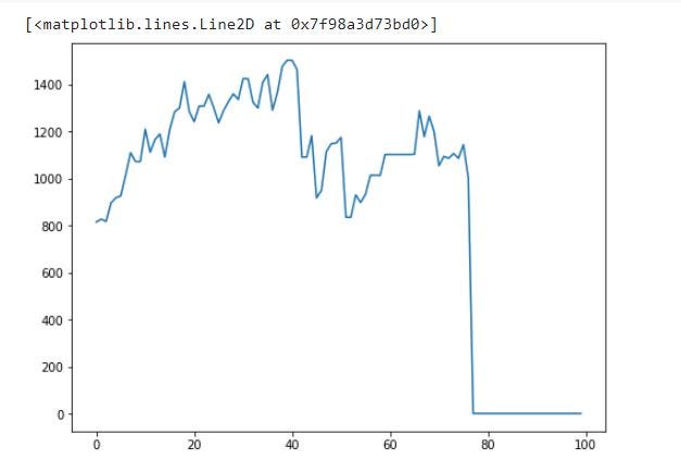
plt.plot(df.generation, df.best_cost)
best_cost of each generation:
plt.figure(figsize=(8, 6))
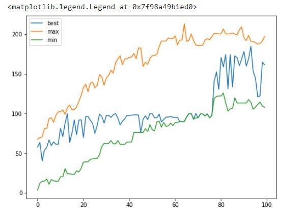
plt.plot(df.generation, df.best_weight, label='best')
plt.plot(df.generation, df.max_weight, label='max')
plt.plot(df.generation, df.min_weight, label='min')
plt.legend()
All weights for each generation:
You can see that cost is 0 after round/generation 79 due to the fact that now all chromosomes/individuals in generations are above the weight limit.
So this is how you can configure your own genetic algorithm and change the function and values as per the need of your problem. I hope this will help you in solving problems from a new perspective.
Comments
Loading comments…