In this article, we are going to discuss and implement one of the most used clustering algorithms: DBSCAN.
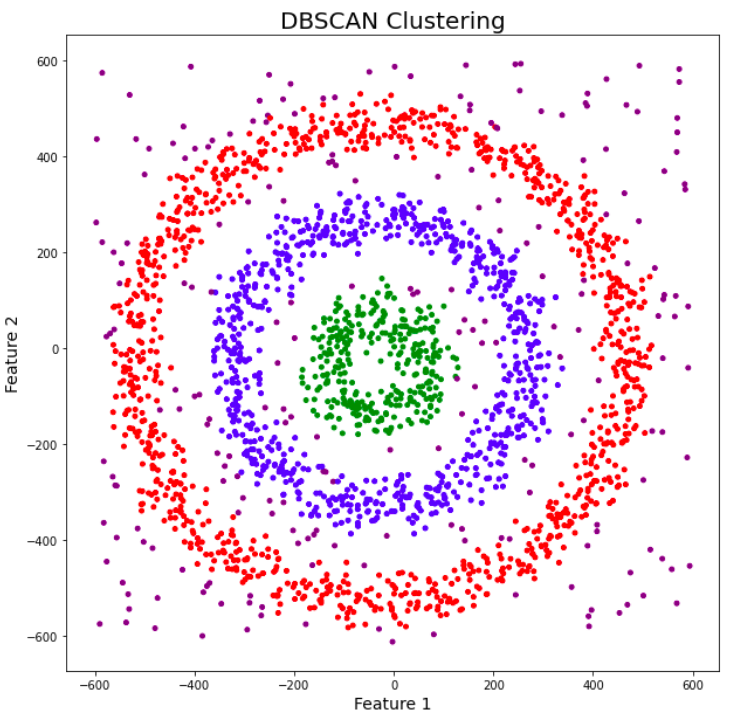
DBSCAN (Density-Based Spatial Clustering of Applications with Noise) is a density-based clustering algorithm that groups together data points that are closely packed (points with many nearby neighbors) while marking them as outliers points in low-density regions. DBSCAN can discover clusters of arbitrary shape, unlike k-means as displayed in the following figure.
The algorithm works by defining two parameters: Eps (a distance threshold) and MinPts (a minimum number of points). The algorithm starts by selecting an arbitrary point from the dataset and retrieves all points within the Eps distance. If the number of points recovered within the eps distance region is greater than MinPts, this point is considered a "core point" and a cluster is created. The algorithm then retrieves all points within the Eps distance of each core point and adds them to the cluster. This process is repeated for all core points until no new points can be added to the cluster. The algorithm then proceeds to the next unvisited point and repeats the process until all points have been visited.
Here is the pseudo-code for DBSCAN Algorithms:
function DBSCAN(data, eps, minPts)
    clusters = []
    for each point in data
        if point is not visited
            mark point as visited
            neighbors = retrieve points within eps distance of point
            if number of neighbors is less than minPts
                mark point as noise cvontim
            else
                create new cluster
                add point to cluster
                add all neighbors to cluster
                for each neighbor in neighbors
                    if neighbor is not visited
                        mark neighbor as visited
                        newNeighbors = retrieve points within eps distance of neighbor
                        if number of newNeighbors is greater than minPts
                            add newNeighbors to neighbors
                add cluster to clusters
    return clusters
Here is a short explanation of each step in the algorithm:
- Initialize an empty list to store the clusters
- Iterate over each point in the data.
2.1. If the point has not been visited yet, mark it as visited.
2.2. Retrieve all points within the Eps distance of the current point
2.3. If the number of neighbors is less than MinPts, mark the point as noise
2.4. If the number of neighbors is greater than MinPts, create a new cluster, add the current point to the cluster and add all of its neighbors to the cluster.
2.5. Iterate over each neighbor in the neighbor's list.
2.6. If the neighbor has not been visited yet, mark it as visited, retrieve its neighbors and check if the number of new neighbors is greater than MinPts, if so, add them to the neighbors' list.
2.7. Add the cluster to the clusters list
- Return the clusters list.
It's important to mention that this is just one way of implementing the DBSCAN algorithm, the actual implementation may vary depending on the programming language and the specific requirements of the problem.
DBSCAN Algorithm Implementation in Python:
The mall customers' data from Kaggle is used for the implementation of the DBSCAN algorithm. You can download the dataset from: https://www.kaggle.com/datasets/vjchoudhary7/customer-segmentation-tutorial-in-python.
Load the necessary libraries and dataset and split the dataset into train and test sets:
import pandas as pd
import numpy as np
import matplotlib.pyplot as plt
import seaborn as sns
%matplotlib inline
#change the path accordngly to csv file. This csv file only has 200 data points
data = pd.read_csv("./archive/Mall_Customers.csv")
# We are taking Age, Annual Income, Spending Score(1-100)
# into consideration and try to find out the cluster
X = data[['Age', 'Annual Income (k$)','Spending Score (1-100)']]
# 80% data for training and remaining 20% for testing
train_set = X.iloc[:160,:]
test = X.iloc[160:,:]
# import DBSCAN from sklearn.cluster
from sklearn.cluster import DBSCAN
# min_samples is number of minpoints, eps is the radius of neighbourhood for any point
dbscan = DBSCAN(eps=12.5, min_samples=4, metric='euclidean')
dbscan.fit(train_set)
x_train = train_set.copy()
# dbscan.labels_ contains the labels assigned to samples of train_set
x_train['cluster'] = dbscan.labels_
# check how many cluster has formed with number of samples belonging to each cluster
x_train['cluster'].value_counts()
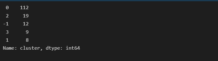
Keep in mind that DBSCAN does not assign a label to points that are considered noise, so the predicted label for such points will be -1.
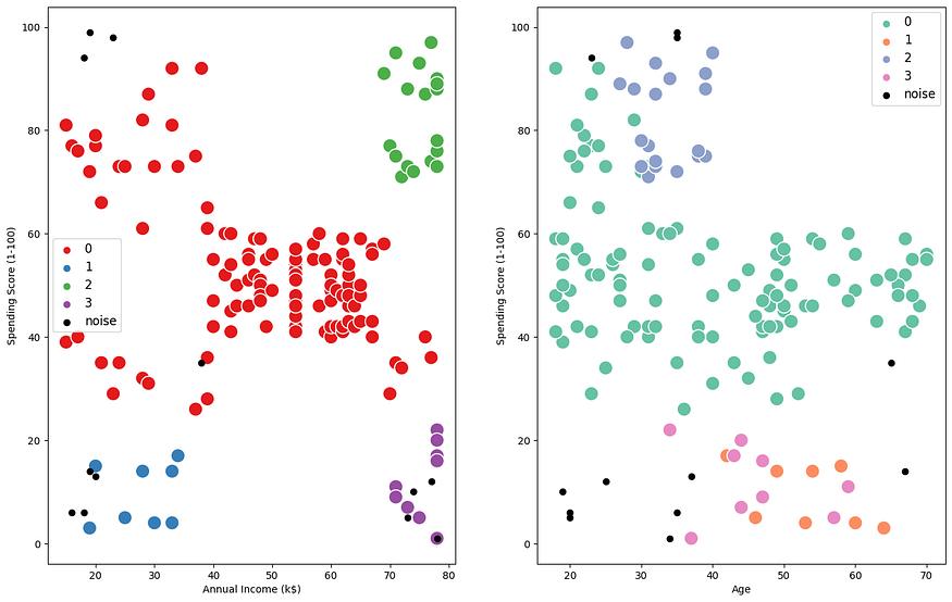
Visualization of created Clusters using SkLearn:
Noise or outliers samples are plotted using black dots.
noise = x_train[x_train['cluster'] == -1]
fig, (ax) = plt.subplots(1,2,figsize = (16,10))
sns.scatterplot(x ='Annual Income (k$)',y ='Spending Score (1-100)',
                data = x_train[x_train['cluster'] != -1], hue = 'cluster', legend = 'full',
                palette='Set1', ax=ax[0], s = 200)
sns.scatterplot(x ='Age',y ='Spending Score (1-100)',
                data = x_train[x_train['cluster'] != -1], hue = 'cluster',
                palette='Set2', ax=ax[1],legend = 'full', s = 200)
ax[0].scatter(x ='Annual Income (k$)',y ='Spending Score (1-100)',
                data = noise, label = 'noise', c ='black')
ax[1].scatter(x ='Age',y ='Spending Score (1-100)',
                data = noise, label = 'noise', c ='black')
ax[0].legend()
ax[1].legend()
plt.setp(ax[0].get_legend().get_texts(), fontsize = '12')
plt.setp(ax[1].get_legend().get_texts(), fontsize = '12')
How do I predict the cluster label for test/new samples from the trained DBSCAN model?
As we know now, In DBSCAN, the cluster assignment of a sample is determined by its distance to nearby samples, as determined by the eps and minsamples parameters. Once the model is trained, you can use the **labels** attribute to obtain the cluster labels for each sample in the test data.
DBSCAN() class function does not have the prediction method to predict clusters for new data points and test samples. Therefore, We can write a custom function to predict the cluster label for new samples using a trained DBSCAN model. The basic idea is to calculate the distance between the new sample and all the samples in the training set, and then find the closest sample that is within the distance threshold defined by the eps parameter. Then you can return the cluster label of that closest sample as the predicted label for the new sample.
from sklearn.metrics import pairwise_distances
import numpy as np
def predict_cluster(dbscan, X_new, metric):
    """ Predicts the cluster label for new samples using a trained DBSCAN model.
    Parameters:
    dbscan: trained DBSCAN model
    X_new: array of new samples,
    metric: the distance criteria used same as used for training the DBSCAN
    shape (n_samples, n_features)
    Returns: array of predicted cluster labels, shape (n_samples,)
    """
    # Calculate pairwise distances between new samples and all samples in the training set
    distances = pairwise_distances(X_new, dbscan.components_, metric=metric)
    # Find the index of the closest sample within eps distance
    closest_sample_indices = np.argmin(distances, axis=1)
    # Get the cluster labels of the closest samples
    closest_sample_labels = dbscan.labels_[closest_sample_indices]
    return closest_sample_labels
test_set = test.copy()
# You can use this function to predict the cluster label of new samples like this-
test_set['cluster'] = predict_cluster(dbscan, test, 'euclidean')
test_set['cluster'].value_counts()
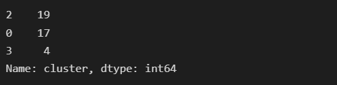 Output of DBSCAN on test_set
It should be noted that This function is using the assumption that the new sample is in the same feature space as the training data. if not, it will give wrong results. Also, this function assumes that the distance metric used for clustering is Euclidean distance.
Hyperparameter Selection For DBSCAN:
How to select the hyperparameters for DBSCAN? The two main hyperparameters in DBSCAN are the "eps" and "min_samples" parameters.
The eps parameter determines the radius around each data point within which a sufficient number of other data points must reside for that point to be considered a core point, and thus included in a cluster. The min_samples parameter specifies the minimum number of data points that must be present within the epsilon radius for a point to be considered a core point. You can plot the Silhouette score for the models trained on various combinations of hyperparameters and select those hyperparameters which give the highest silhouette score.
Here's an example of using the sklearn library for finding the best parameters for DBSCAN:
from sklearn.metrics import silhouette_score
from sklearn.cluster import DBSCAN
# min_samples is number of minpoints, eps is the radius of neighbourhood for any point
silhouette_ =[]
eps_ = [12,11,10.5,10,9]
min_samples_ = [3,4,5,6,7]
for eps, min_samples in zip(eps_,min_samples_ ):
    dbscan = DBSCAN(eps=eps, min_samples=min_samples)
    dbscan.fit(train_set)
    x_train = train_set.copy()
    x_train['cluster'] = dbscan.labels_
    labels = x_train['cluster']
    silhouette_.append(silhouette_score(train_set, labels))
plt.plot(eps_, silhouette_,'-gD')
plt.xlabel('EPS')
plt.ylabel("Silhouette Score")
plt.title("Eps Vs. Silhoutte Score")
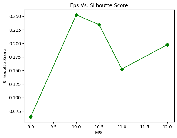
From the above graph, it is evident that the best silhouette score is achieved when the eps is equal to 10 and min_samples = 5. Therefore, we can train our model for these hyperparameters.
Note that here we are using silhouette score as a metric to evaluate the performance of the model. you can also use other metrics like the Davies-Bouldin index, CH index and etc.
Pros of DBSCAN:
-DBSCAN can discover clusters of arbitrary shape, unlike k-means.
-It is robust to noise, as it can identify points that do not belong to any cluster as outliers.
-It does not require the number of clusters to be specified in advance.
Cons OF DBSCAN:
-It is sensitive to the choice of the Eps and MinPts parameters.
-It does not work well with clusters of varying densities.
-It has a high computational cost when the number of data points is large.
-It is not guaranteed to find all clusters in the data.
DBSCAN is a useful algorithm for clustering data that has a spatial or density-based structure. It is beneficial for discovering clusters in large, complex datasets where the number of clusters is not known in advance. However, it does have some limitations and its performance can be sensitive to the choice of parameters.
You can also have a look at the following articles:
- Statistics Series for Data Science
- All About Python : You Must Know
- Let's Explore Postgres in Deep
Thanks for taking out the time to read this article. I have tried to include all the points related to the DBSCAN algorithm. Please share your thoughts on using the DBSCAN algorithm and its performance. If you have enjoyed reading the article, feel free to clap and appreciate it. Stay tuned for future articles.
Comments
Loading comments…