Logistic regression is a regression analysis used when the dependent variable is binary categorical. Target is True or False, 1 or 0. However, although the general usage is binary, it is also possible to make multi-class classifications by making some modifications.
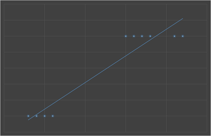
We fit a straight line to the data in linear regression. If our dependent variable, that is, our target variable, has a binary type, drawing a straight line here will not estimate a fine result. In such cases, it would be right to calculate the probabilities.
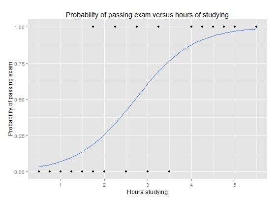
Logistic regression uses an s-shaped curve (a logistic function) instead of a linear line. Although it is a probability function and yields a probability value, logistic regression is used for classification. It returns 1 if the probability is above 0.5 (50%) and 0 if it is below. Just like multiple linear regression, more than one independent variable can be included in the model. Likewise, it can work with both continuous variables and discrete, categorical variables as independent variables.
Just like linear regression, logistic regression also uses gradient descent. In addition to this, we can also use maximum likelihood.
Maximum-likelihood
The purpose here is to find the parameters of a given data. We will find such parameters that will maximize the likelihood. It estimates a parameter and this parameter is a constant variable. The ultimate goal is to find this parameter and fit the most appropriate distribution on the data by using this parameter(s). There are different types of distributions such as normal, exponential, gamma, Poisson, etc. When you fit one of these distributions on top of the data, it will be easier to explain and use the data.
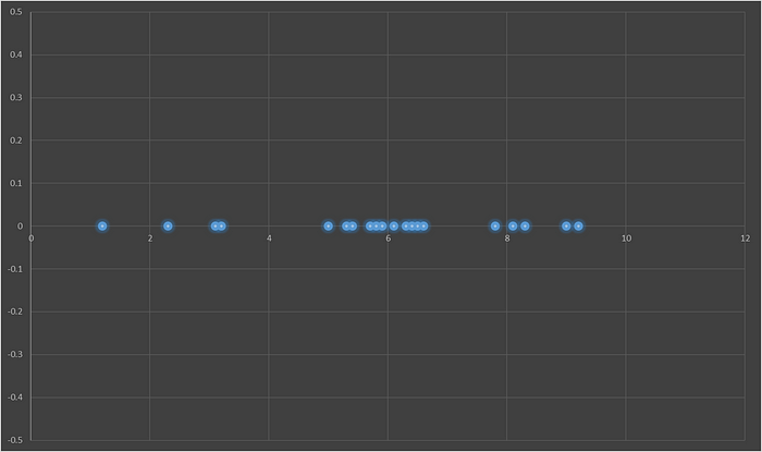
Let's say we measured the minute of the first corner in 20 different Champions League football matches. We should find the best fit distribution over this data. We will use the normal distribution which comes to mind first (and also, as we recognize when we look at the data).
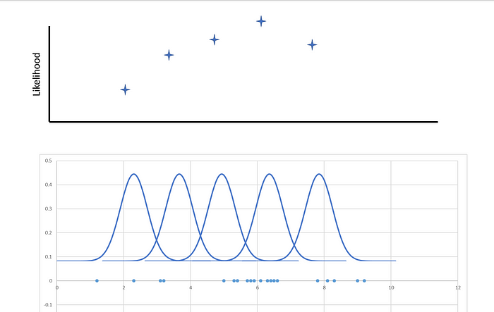
We are trying to find the best distribution that gives the maximum likelihood. We have two parameters in normal distributions, mean and standard deviation. Then, our goal is to find the mean and standard deviation that will give the maximum likelihood.
The math here to calculate the likelihood of distributions is another topic. So, I will leave the maximum likelihood subject here and return to logistic regression. As it can be understood, there is a similar approach when fitting the s-shaped curve in logistic regression.
We will first re-code the logistic regression from scratch. At the end of the article, you can find the sklearn implementation.
You can reach the code from this Kaggle notebook.
Logistic Regression Class in Python
Data
We will use Bank Marketing Data Set as data in this demonstration. Since our focus here is the implementation of logistic regression, we will not waste any time on any descriptive or exploratory analysis steps. All numeric features are standard scaled and categorical features are label encoded for simplicity.
Data preparation class:
import pandas as pd
import numpy as np
from sklearn.preprocessing import LabelEncoder, StandardScaler

class Data:

    def __init__(self,path,target):
        self.df = pd.read_csv(path,delimiter=";")
        self.encode()
        self.y = self.df[target].values.reshape(-1,1)
        self.df.drop([target],axis=1,inplace=True)

    def encode(self):
        #feature types
        features = self.__feature_categorization(self.df)
        #categorical > labelencoding
        for f in features["Categorical"]:
            self.label_encoding(f)
        #numerical
        for f in features["Numerical"]:
            self.standard_scaling(f)

    def get_df(self):
        return self.df, self.y

    def check_missing_values(self):
        print(self.df.isnull().sum())
        return True

    def label_encoding(self,col):
        self.df[col] = self.df[col].astype(str)
        le = LabelEncoder()
        x = self.df[col].values.reshape(-1,1)
        le.fit(x)
        x_label_encoded = le.transform(x).reshape(-1,1)
        self.df[col] = x_label_encoded.reshape(len(x_label_encoded),1)
        return True

    def standard_scaling(self,col):
        x = self.df[col].values.reshape(-1,1)
        scaler = StandardScaler()
        scaler.fit(x)
        self.df[col] = scaler.transform(x)
        return True

    def __feature_categorization(self,df):
        numerical = df.select_dtypes(include=[np.number]).columns.values.tolist()
        categorical = df.select_dtypes(include=['object']).columns.values.tolist()
        datetimes = df.select_dtypes(include=['datetime',np.datetime64]).columns.values.tolist()
        features = {"Numerical":numerical,"Categorical":categorical,"Datetimes":datetimes}
        return features
path = PATH
D = Data(path,"y")
df, y = D.get_df()
We have implemented the data processing step in the above class. Since there were no missing values in the bank data set we used, no generic action was taken in class in such a manner.
Encoding method:

In the above method, we first determine the types of all the features in the dataframe. Then, standard scaling is applied to numerical features and label encoding is applied to categorical features.
Model
Logistic regression class:
class LogisticRegression:
def __init__(self,epoch=50000,lr=0.001,method="gradient"):
self.epoch = epoch
self.lr = lr
self.w = None
self.b = None
self.method = method
self.cost_list = []
def fit(self,X,y):
#initialization
X, self.w = self.__initialization(X)
#iterations
for i in range(self.epoch):
#prediction
z = self.__get_z(X)
#sigmoid
a = self.__sigmoid(z)
#calculate lost
#gradient
if self.method == "gradient":
cost = self.__calculate_loss(a, y)
self.cost_list.append(cost)
gr = self.__gradient_descent(X, a, y)
elif self.method == "likelihood":
l = self.__log_likelihood(X,y)
self.cost_list.append(l)
gr = self.__gradient_l(X, a, y)
#update w
self.w = self.__update(self.w, gr)
self.b = X[:,0]
return True
def predict(self,X):
b = np.ones((X.shape[0],1))
X = np.concatenate((b,X),axis=1)
z = self.__get_z(X)
s = self.__sigmoid(z)
result = [1 if x >=0.5 else 0 for x in s]
return result
def get_cost(self):
return self.cost_list
def __get_z(self,X):
return np.dot(X,self.w)
def __sigmoid(self,z):
return 1 / (1 + np.exp(-z))
def __gradient_descent(self,X,a,y):
return np.dot(X.T,(a-y)) / y.shape[0]
def __update(self,w,gr):
return w - self.lr * gr
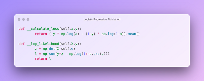
def __calculate_loss(self,a,y):
return (-y * np.log(a) - (1-y) * np.log(1-a)).mean()
def __initialization(self,X):
b = np.ones((X.shape[0],1))
X = np.concatenate((b,X),axis=1)
w = np.zeros(X.shape[1]).reshape(-1,1)
return X,w
def __log_likelihood(self,X,y):
z = np.dot(X,self.w)
l = np.sum(y*z - np.log(1+np.exp(z)))
return l
def __gradient_l(self,X,a,y):
return np.dot(X.T,y-a)
A logistic regression model can be fitted and predictions can be conducted using the above class. Let's take a look at piece by piece.
Fit Method:
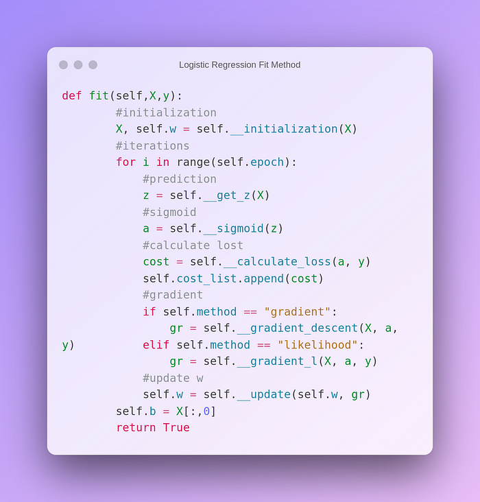
Firstly we initialize weights and bias. Bias will be all ones with the size of the input and we add them as a constant part of X. Weights will be zeros.
Initialization:

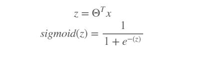
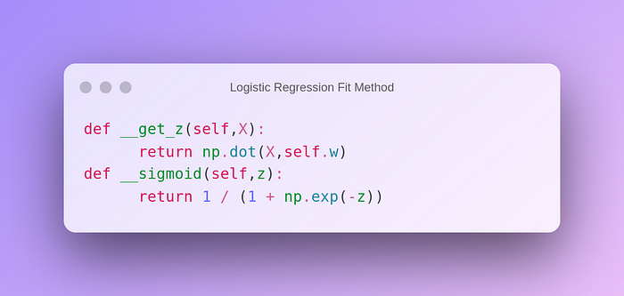
Then the sigmoid function is calculated by predicting with weights and input.
Sigmoid function:
Sigmoid method:
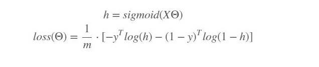
Later, we calculate losses and append them into a list, (or maximum likelihood).
The loss function of logistic regression:
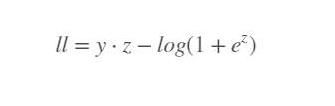
Maximum likelihood:
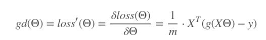
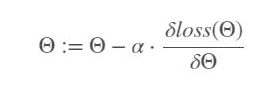
Our goal was to minimize loss by updating weights, (called fitting). To achieve this, we use the gradient descent method. It is the derivative of loss with respect to weights. With this value, we update weights in each epoch.
Gradient descent:
Gradient Descent Method:

Finally, we can predict test data and check the confusion matrix to evaluate our model.
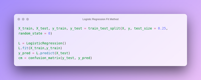
Confusion Matrix:

Not a bad result for a generic model.
Sklearn Implementation
from sklearn.linear_model import LogisticRegression
Parameters;
penalty: 'none': no penalty; 'l2': add L2 penalty; 'l1': add an L1 penalty, 'elasticnet': both L1 and L2 penalty terms are added.
dual: If your n_sample > n_feature, then prefer False. If it is set as True, you can only implement L2 penalty with liblinear solver.
tol: It is tolerance for stopping criteria. default = 1e-4
C: It must be a positive float. It is the inverse of regularization strength (1 / lambda). Higher C means less regularization. default = 1.0
fit_intercept: Do you want to add a constant as we did above? default = True
intercept_scaling: It's useful if you use 'liblinear' solver and if fit_intercept is also True. You can scale intercept value. default = 1
class_weight: You can give weights in dictionary type. Or you can use the “balanced” mode to automatically adjust weights proportionally inverse of the class frequencies. default = None
random_state: Determine randomness
solver: Choices are : {'newton-cg', 'lbfgs', 'liblinear', 'sag', 'saga'}, default = 'lbfgs'
liblinear is a good choice in the case of small datasets. 'sag' and 'saga' are the faster ones for large datasets. If your case is a multiclass classification you can only use 'newton-cg', 'sag', 'saga', and 'lbfgs'. Not all types work with all regularization parameters.
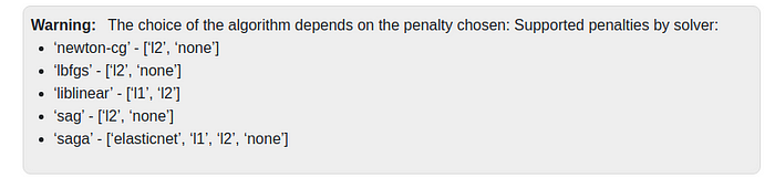
Copied the above from sklearn documentation.
max_iter: maximum number of iterations. default = 100
multi_class: Choices are: {'auto', 'ovr','multinomial'}, default = “auto”. ovr is for a binary problem. You cannot use multinomial if the solver is liblinear.
verbose: logging parameter**.**
warm_start: Set True if you want to reuse the previous solution.
n_jobs: Run in parallel, how many CPUs?
l1_ratio: l1 regularization hyperparameter.
Attributes:
classes : class labels of the classifier.
coef : coefficients.
intercept: intercept
nfeatures_in : how many features are used in fit?
featurenames_in : the names of features used in the fit.
niter: actual number of iterations.
Below, you can find sklearn implementation of logistic regression with GridSearchCV hyper-parameter tuning. With the help of GridSearch, you select the best parameters for your case.
Sklearn Implementation with Gridsearch:
from sklearn.linear_model import LogisticRegression
from sklearn.model_selection import GridSearchCV

params = {"penalty":["none","l1","l2","elasticnet"],
          "C": np.logspace(-5,5,20),
          "solver":["liblinear","sag","saga","lbfgs","newton-cg"],
          "max_iter": [10,100,1000,10000,100000]
    }
model = LogisticRegression(random_state=0)
clf = GridSearchCV(model, param_grid = params, cv = 5, n_jobs=-1)
clf.fit(X_train,y_train)
best_params = clf.best_params_
best_model = LogisticRegression(**best_params)
best_model.fit(X_train, y_train)
y_pred = clf.predict(X_test)
cm_sk = confusion_matrix(y_test, y_pred)
Conclusion
Logistic regression can be used for classification problems. It can be used for different types of features. It will work for cases that are not very complex. It can also be used as a starting model in very complex situations. It is useful to note the logistic regression code snippets somewhere.
Comments
Loading comments…