Image Stitching Using OpenCV

Welcome to our second image stitching tutorial part, where we’ll finish our first tutorial part, and we’ll receive our stitched image.

So here is the list of steps from our first tutorial on what we should do to get our final stitched result:

1. Compute the sift-key points and descriptors for left and right images;
2. Compute distances between every descriptor in one image and every descriptor in the other image;
3. Select the top best matches for each descriptor of an image;
4. Run RANSAC to estimate homography;
5. Warp to align for stitching;
6. Finally, stitch them together.

In our first tutorial, we did the most job. We finished three first steps in our previous tutorial, so the last 3 steps are left to do. What is left is just several lines of code.

So, once we have obtained the best matches between the images, our next step is to calculate the homography matrix. As we described before, the homography matrix will be used with the best matching points to estimate a relative orientation transformation within the two images.

To estimate the homography in OpenCV is a simple task. It’s one line of code:

H, __  =  cv2.findHomography(srcPoints, dstPoints, cv2.RANSAC, 5)

Before starting the coding stitching algorithm, we need to swap image inputs. So “img_” will take the right image, and “IMG” will take the left image.

So let’s jump into stitching coding:

MIN_MATCH_COUNT = 10
if len(good) > MIN_MATCH_COUNT:
    src_pts = np.float32([ kp1[m.queryIdx].pt for m in good ]).reshape(-1,1,2)
    dst_pts = np.float32([ kp2[m.trainIdx].pt for m in good ]).reshape(-1,1,2)

    M, mask = cv2.findHomography(src_pts, dst_pts, cv2.RANSAC,5.0)

    h,w = img1.shape
    pts = np.float32([ [0,0],[0,h-1],[w-1,h-1],[w-1,0] ]).reshape(-1,1,2)
    dst = cv2.perspectiveTransform(pts,M)

    img2 = cv2.polylines(img2,[np.int32(dst)],True,255,3, cv2.LINE_AA)
    cv2.imshow("original_image_overlapping.jpg", img2)
else:
    print ("Not enough matches are found - %d/%d" % (len(good),MIN_MATCH_COUNT))

So at first, we set our minimum match condition count to 10 (defined by MIN_MATCH_COUNT), and we only do stitching if our good match exceeds our required matches. Otherwise, show a message saying not enough matches are present.

So in the if statement, we are converting our Keypoints (from a list of matches) to an argument for the findHomography() function. I can’t explain this in detail because I didn’t have time to chatter about this, and there is no use for that.

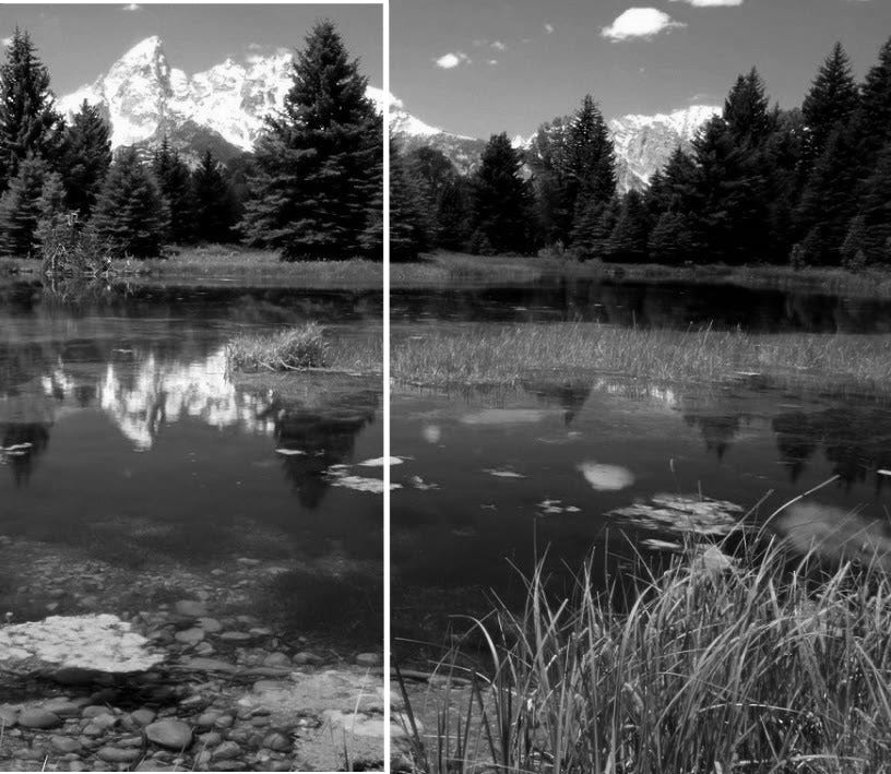
Simply talking in this code line cv2.imshow("original_image_overlapping.jpg", img2), we are showing our received image overlapping area:

So, once we have established a homography, we need to warp perspective, essentially changing the field of view. We apply the following homography matrix to the image:

warped_image = cv2.warpPerspective(image, homography_matrix, dimension_of_warped_image)

So we use this as follows:

dst = cv2.warpPerspective(img_,M,(img.shape[1] + img_.shape[1], img.shape[0]))
dst[0:img.shape[0], 0:img.shape[1]] = img

In the above two lines of code, we are taking overlapping areas from two given images. Then in “DST”, we have received only the right side of the image that is not overlapping, so in the second line of code, we place our left side image to the final image. So at this point, we have a fully stitched image:

So from this point, what is left is to remove the dark side of the image, so we’ll write the following code to remove the black font from all image borders:

def trim(frame):
    #crop top
    if not np.sum(frame[0]):
        return trim(frame[1:])
    #crop bottom
    elif not np.sum(frame[-1]):
        return trim(frame[:-2])
    #crop left
    elif not np.sum(frame[:,0]):
        return trim(frame[:,1:])
    #crop right
    elif not np.sum(frame[:,-1]):
        return trim(frame[:,:-2])
    return frame

And here is the final defined function we call to trim borders, and at the same time, we show that image on our screen. If you want, you can also write it to disk:

cv2.imshow("original_image_stiched_crop.jpg", trim(dst))
#cv2.imwrite("original_image_stiched_crop.jpg", trim(dst))

With the above code, we’ll receive the original image as in the first place:

Here is the complete final code:

import cv2
import numpy as np

img_ = cv2.imread('original_image_right.jpg')
#img_ = cv2.imread('original_image_left.jpg')
#img_ = cv2.resize(img_, (0,0), fx=1, fy=1)
img1 = cv2.cvtColor(img_,cv2.COLOR_BGR2GRAY)

img = cv2.imread('original_image_left.jpg')
#img = cv2.imread('original_image_right.jpg')
#img = cv2.resize(img, (0,0), fx=1, fy=1)
img2 = cv2.cvtColor(img,cv2.COLOR_BGR2GRAY)

sift = cv2.xfeatures2d.SIFT_create()
# find key points
kp1, des1 = sift.detectAndCompute(img1,None)
kp2, des2 = sift.detectAndCompute(img2,None)

#cv2.imshow('original_image_left_keypoints',cv2.drawKeypoints(img_,kp1,None))

#FLANN_INDEX_KDTREE = 0
#index_params = dict(algorithm = FLANN_INDEX_KDTREE, trees = 5)
#search_params = dict(checks = 50)
#match = cv2.FlannBasedMatcher(index_params, search_params)
match = cv2.BFMatcher()
matches = match.knnMatch(des1,des2,k=2)

good = []
for m,n in matches:
    if m.distance < 0.03*n.distance:
        good.append(m)

draw_params = dict(matchColor=(0,255,0),
                       singlePointColor=None,
                       flags=2)

img3 = cv2.drawMatches(img_,kp1,img,kp2,good,None,**draw_params)
#cv2.imshow("original_image_drawMatches.jpg", img3)

MIN_MATCH_COUNT = 10
if len(good) > MIN_MATCH_COUNT:
    src_pts = np.float32([ kp1[m.queryIdx].pt for m in good ]).reshape(-1,1,2)
    dst_pts = np.float32([ kp2[m.trainIdx].pt for m in good ]).reshape(-1,1,2)

    M, mask = cv2.findHomography(src_pts, dst_pts, cv2.RANSAC, 5.0)

    h,w = img1.shape
    pts = np.float32([ [0,0],[0,h-1],[w-1,h-1],[w-1,0] ]).reshape(-1,1,2)
    dst = cv2.perspectiveTransform(pts, M)
    img2 = cv2.polylines(img2,[np.int32(dst)],True,255,3, cv2.LINE_AA)
    #cv2.imshow("original_image_overlapping.jpg", img2)
else:
    print("Not enought matches are found - %d/%d", (len(good)/MIN_MATCH_COUNT))

dst = cv2.warpPerspective(img_,M,(img.shape[1] + img_.shape[1], img.shape[0]))
dst[0:img.shape[0],0:img.shape[1]] = img
cv2.imshow("original_image_stitched.jpg", dst)

def trim(frame):
    #crop top
    if not np.sum(frame[0]):
        return trim(frame[1:])
    #crop top
    if not np.sum(frame[-1]):
        return trim(frame[:-2])
    #crop top
    if not np.sum(frame[:,0]):
        return trim(frame[:,1:])
    #crop top
    if not np.sum(frame[:,-1]):
        return trim(frame[:,:-2])
    return frame

cv2.imshow("original_image_stitched_crop.jpg", trim(dst))
#cv2.imsave("original_image_stitched_crop.jpg", trim(dst))

Conclusion

These tutorials taught us how to implement and perform image stitching and panorama construction using OpenCV and wrote a final code for image stitching.

To stitch images with our algorithm, it’s required to do four main steps:

1. detecting key points and extracting local invariant descriptors;
2. get matching descriptors between images;
3. apply RANSAC to estimate the homography matrix;
4. apply a warping transformation using the homography matrix.

This algorithm works well in practice when constructing panoramas only for two images.