When dealing with time-series data, it has a different format and usually has a DateTime index and its corresponding value. Some examples of time-series data can be stock market data, count of sunspots, or temperature reading of the atmosphere.
In this article, I will take you through the different Pandas methods that can be used with time-series stock data.

Understanding datetime index
When dealing with time-series data, date and time information is a must and is always given. But the date and time information is not always in columns separated. There is a possibility that it is actually the index of a dataset (datetime index). So let's see how Pandas can help us deal with such situations.
Importing packages
We will start off by importing the necessary libraries and packages. The numpy and pandas libraries are imported for dealing with the data. For visualization, matplotlib is imported. Python's built-in library ‘datetime' library is imported too.
>>> import numpy as np
>>> import pandas as pd
>>> import matplotlib.pyplot as plt
>>> %matplotlib inline
>>> from datetime import datetime
Creating a datetime object
Now we will initialize variables of year, month, day, hour, minute and second and then create a datetime object.
>>> yr = 2020
>>> mn = 1
>>> day = 6
>>> hr = 15 #24 hour format
>>> mins = 14
>>> sec = 6
>>> date = datetime(yr,mn,day,hr,mins,sec)
>>> date
datetime.datetime(2020, 1, 6, 15, 14, 6)
One thing to keep in mind is that this datetime object has the datatype ‘datetime'.
>>> type(date)
datetime.datetime
Now from this datetime datatype, many attributes can be grabbed as shown below.
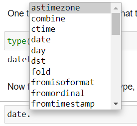
Source: Author
>>> date.month
1
>>> date.hour
15
Datetime list
>>> l1 **=** [datetime(2020,1,1),datetime(2020,1,2)]
>>> l1
[datetime.datetime(2020, 1, 1, 0, 0), datetime.datetime(2020, 1, 2, 0, 0)]
>>> type(l1)
list
Now we can convert this list into an index.
>>> l1_indx **=** pd.DatetimeIndex(l1)
>>> l1_indx
DatetimeIndex(['2020-01-01', '2020-01-02'], dtype='datetime64[ns]', freq=None)
Now this index form that you see is how the datetime is mentioned in the time series dataset.
Time series dataframe
Now let's create a dummy dataframe with the datetime index.
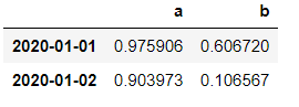
>>> df **=** np.random.rand(2,2)
>>> df
array([[0.97590609, 0.60672033],
       [0.90397291, 0.106567  ]])
>>> cols=['a','b']
>>> dataset = pd.DataFrame(df,l1_indx,cols)
dataset
We can call many methods on these indexes like finding the max or min of the index.
>>> dataset.index.max()
Timestamp('2020-01-02 00:00:00')
>>> dataset.index.min()
Timestamp('2020-01-01 00:00:00')
Resampling of time
Now that we have understood the importance and usage of datetime index. The next thing to understand is the resampling of time. Usually, the datasets which have datetime index are mentioned on a smaller scale. That is each row in the dataset corresponds to a day, hour, or minute. But to understand the data better, at times it's better to just aggregate the data. This is done based on some frequency like monthly, quarterly or half-yearly. This is where pandas come into the picture. With its frequency sampling tools, these functions can be easily performed.
To understand this concept practically, we will perform sampling on a stock data. The link is provided at the end of the article.
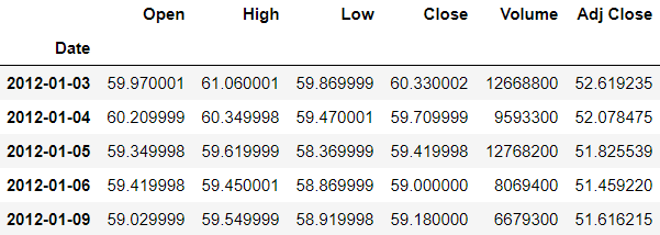
Reading of data
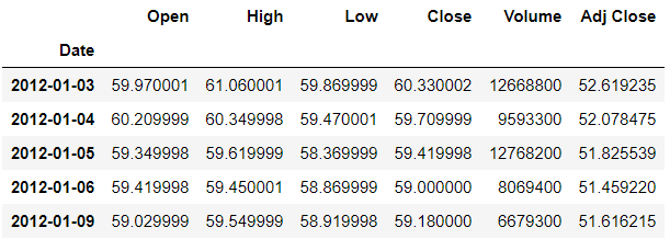
>>> df = pd.read_csv('stocks.csv')
>>> df.head()
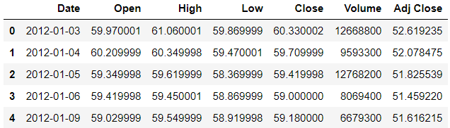
So the date column has to be converted into the index. But before we convert it, we need to check the datatype. Currently, the datatype is an object but we need to change it into datetime datatype.
>>> df.info()
<class 'pandas.core.frame.DataFrame'>
RangeIndex: 1258 entries, 0 to 1257
Data columns (total 7 columns):
 #   Column     Non-Null Count  Dtype
---  ------     --------------  -----
 0   Date       1258 non-null   object
 1   Open       1258 non-null   float64
 2   High       1258 non-null   float64
 3   Low        1258 non-null   float64
 4   Close      1258 non-null   float64
 5   Volume     1258 non-null   int64
 6   Adj Close  1258 non-null   float64
dtypes: float64(5), int64(1), object(1)
memory usage: 68.9+ KB
>>> df.Date = pd.to_datetime(df.Date)
>>> df.info()
<class 'pandas.core.frame.DataFrame'>
RangeIndex: 1258 entries, 0 to 1257
Data columns (total 7 columns):
 #   Column     Non-Null Count  Dtype
---  ------     --------------  -----
 0   Date       1258 non-null   datetime64[ns]
 1   Open       1258 non-null   float64
 2   High       1258 non-null   float64
 3   Low        1258 non-null   float64
 4   Close      1258 non-null   float64
 5   Volume     1258 non-null   int64
 6   Adj Close  1258 non-null   float64
dtypes: datetime64[ns](1), float64(5), int64(1)
memory usage: 68.9 KB
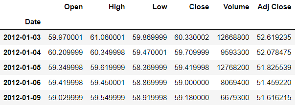
Now we will make the Date column as the index.
>>> df.set_index('Date',inplace=True)
>>> df.head()
Another short way of converting the dates into datetime object and also making them the index is to mention the index column and parsing value as true while reading the csv file. The parse_dates argument will automatically parse the dates as datetime object.
>>> df = pd.read_csv('stocks.csv',index_col='Date',parse_dates=True)
Resampling
By calling the resample() method on the dataframe, we can do the sampling. The argument it takes is rule-how you want to resample. Here we will use ‘A' which resamples based on the end of the year and perform some aggregation operation. Some of the rules are given below:
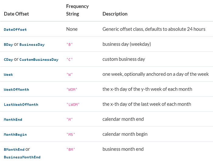
Source: Author
You can find the entire list here:
Time series / date functionality - pandas 1.2.0 documentation
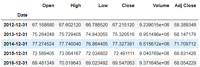
>>> df.resample(rule='A').mean()
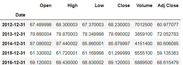
We can also create our own aggregate function. Like extracting the last entry of the year.
>>> def last(entry):
    return entry[-1]
>>> df.resample(rule='A').apply(last)
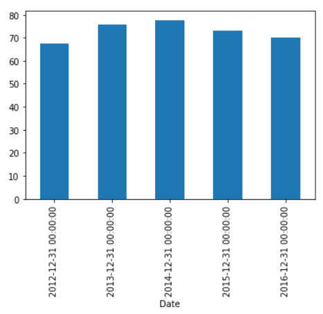
Plotting
Now we can plot the individual columns based on some frequency according to our needs.
>>> df['High'].resample('A').mean().plot(kind='bar')
Shifting of time
At times, we need to move our forward back or forth with a certain amount of time steps, this is called time-shifting. Pandas have the necessary methods to help us do this. The shift() method helps in doing this. It takes the argument period — which is the no. of periods we want to shift with. So if we mention the period as 1, the row values will shift one down.
>>> df.head()
>>> df.shift(periods=1).head()
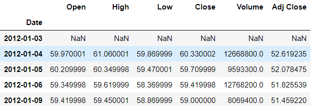
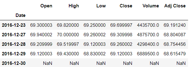
So the first row has null values and the row values are shifted one down. To shift it upwards, we mention the negative value of the period.
>>> df.tail()
>>> df.shift(periods=-1).tail()
Now let's look into how to shift the index instead of the data. In case, you want to change all the days in a particular month to the same-day value, it can be done using the tshift() method. By mentioning the frequency argument, the changes can be made.
In the dataframe, we will try to change all the days of a particular month to have the same day.
>>> df.head()
>>> df.tshift(freq='M').head()
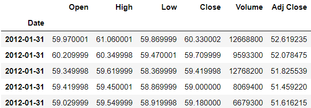
Now you can see that all the days in the first month of January is 31st.
Rolling and expanding of data
The time-series data especially financial data can be noisy at times which can give issues while recognizing a pattern. So by rolling the data based on some function like mean we can get a general trend idea. Rolling is also referred to as the moving average.
We will set a window for a time interval and then perform the aggregate function on that interval.
We will plot the data so as to understand the difference when it is rolled.
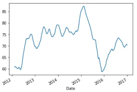
>>> df.Open.plot()
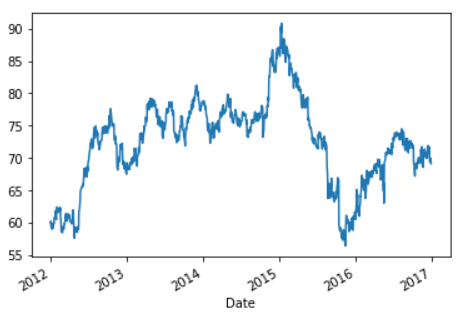
Now as you can see above, there is a lot of noise since it the daily data. So what we can do is average the data (rolling mean/moving average) for a window of a week.
The rolling() method is used and the window argument is passed which is the size of the moving window. So we will mention it as 7, since we want it for a week.
>>> df.rolling(7).mean().head(9)
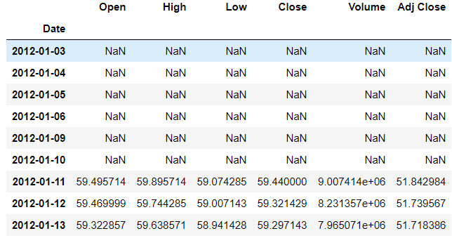
Now the first 6 rows are empty because there wasn't enough data to fill the value. The 7th row's value is the average of the first 7 rows values. The 8th row has the value of the average of itself and the previous 6 rows and so on.
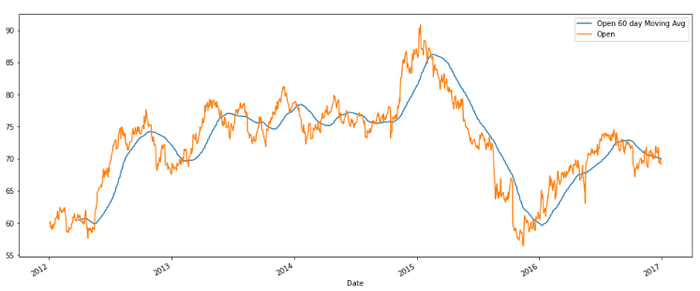
Now we will plot the rolled data and see the difference. We will take the window as 30 days.
>>> df.rolling(30).mean()['Open'].plot()
Now you can see that this plot has less noise compared to the previous one and the trend can be seen in a better way.
>>> df['Open 60 day Moving Avg'] = df.Open.rolling(60).mean()
>>> df[['Open 60 day Moving Avg','Open']].plot(figsize=(17,7))
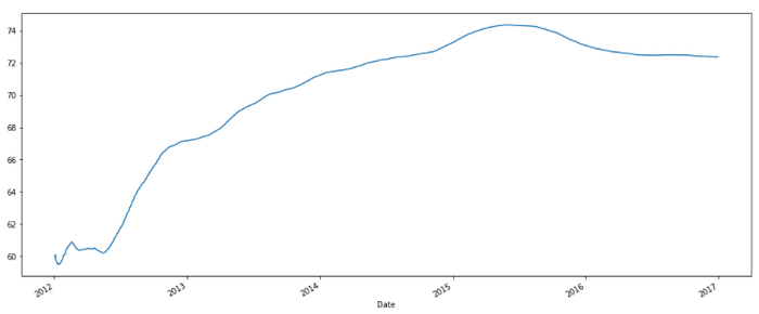
Now suppose you want to take everything from the beginning of the time-series data to that time step for analysis, this can be done by the expanding function.
The expanding() function takes the argument of min_periods which is the value of the minimum period. So what this does is, for a particular time step, it takes the value of all the previous values and averages it out.
>>> df['Open'].expanding().mean().plot(figsize=(17,7))
Refer to the notebook for code here.
Link to dataset here.
Reach out to me: LinkedIn
Check out my other work: GitHub
Comments
Loading comments…