Molecular Dynamics: Velocity Verlet

Molecular dynamics (MD) is an extremely popular technique that is used to, among other things, simulate motion of atoms or molecules. A variety of fields have adopted MD, including micromechanics, biophysics, and chemistry. One of the reasons for MD’s cross-discipline nature is its relative simplicity and robustness. There are a large number of open-source or free access libraries for MD including LAMMPS, MDAnalysis, and MDTraj — making design and implementation of MD as simple as mounting a library and outlining the simulation parameters.

Despite the readily accessible open source libraries, it’s extremely important to understand the roots of MD as a modeling technique to make sense of its results, build simulations, and understand MD’s limitations. Without going into full detail about the numerical derivations of MD (there are many great textbooks), I’ll help derive and demonstrate one of the most popular position integration algorithms: Velocity Verlet.

What is “position integration”?

Simply put, position integration in MD is the process used to find the direction and distance particles move given some time-step. Knowing how groups of particles/molecules/atom’s positions change over time given some external stimulus (e.g. force, electric field), can typically provide all the necessary physical information to understand structural, thermodynamic, or flow properties.

Origins of Velocity Verlet Integration

Our starting point will be a generalized graph indicating a particle’s position (r) with respect to time (t).

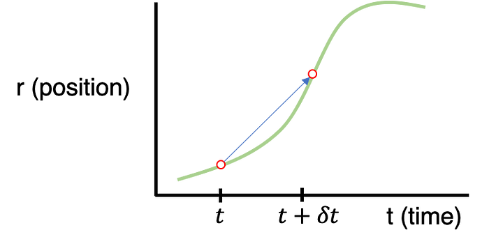
What we’re interested in is how to extrapolate the particle’s next position given all the information about the rest of the system (e.g. external stimulus, positions of all other particles, etc.). In short, we need to find the relationship between r(t) and r(t+dt) where dt is the time-step between iterations. If we assume that the dt step between t and t+dt is small, we can approximate the expression for r(t+dt) using a Taylor expansion:

The O(dt⁴) is term an error value that encompasses the trailing error due to ignoring dt⁴, dt⁵, dt⁶, etc. contributions. Here, the “over dots” represent the first, second, and third time derivatives with respect to position. More familiar expressions for this notation could be the following:

For simplicity, I’m going to stick with the over-dot notation during the Velocity Verlet derivation until the final expression.

Returning to Eq. 1, we can rearrange the equation to express the finite difference in position between r(t) -> r(t + dt):

This is also referred to as the “Forward Euler” expression, in that the position derivative is calculated moving from r(t) -> r(t +dt). Conversely, we can also use the “Backward Euler” expression by calculating the derivative moving from r(t-dt) -> r(t).

Then, if we subtract Eq. 3 from Eq. 2 (Equation 3- Equation 2):

and then simplify, solving for r(t + dt), we get:

Eq. 4 is the expression for the Verlet position integrator — which is a position-update algorithm. However, it is not self-starting. If you imagined a simulation starting at t=0, it would need to know the position at t=-dt to begin the simulation.

To improve on this, we must first find an appropriate expression for velocity. This can be done by following a similar algebraic procedure as before, and add Eq. 3 to Eq. 2 (Equation 3 + Equation 2) and solve for the velocity (first time-derivative of position).

Eq. 5 can be rearranged to solve for r(t-dt), which takes the form of:

We can then plug the above for r(t-dt) into the Verlet position integrator (Eq. 4) and simplify to the form of:

The above expression is the final form of the Velocity Verlet position integrator. By substituting in more familiar terms for the over-dot notation we’re left with:

Here we can see that all we need to know to update the position is the current position, velocity, force, mass, and time-step. Unlike the Verlet integrator, the Velocity Verlet is self-starting because no prior knowledge of the system’s prior state is needed to move it forward.

The velocity integrator for the Verlet Verlet algorithm can be extracted by first substituting (t+dt) for (t) terms in Eq. 5 and Eq.4, and then substituting in Eq. 4 for the r(t+2dt) term in Eq. 5, we’re left with:

Or, an equivalent form that is often used:

Equation 6 and 7 are the Velocity Verlet integrators for position and velocity. As you might notice, the r(t+dt) position must be defined before the v(t+dt) velocity is defined. It is only sensible then, that the update of the position must happen before the update to velocity. With this in mind, there is a traditional sequence of steps that are typically used when performing a molecular dynamics simulation. Something along the lines of:

1. Update All positions
2. Update All Forces
3. Update All velocities
4. Apply boundary conditions (including temperature, pressure controls)
5. Move global time forward by time-step (dt)
6. Calculate any output
7. Repeat step 1–6 as many times as necessary

Many other considerations that must be taken when using MD, including; how periodic boundary conditions are implemented, optimizing computation speed using neighbor lists or cell meshes, and general limitations of usage. But proper use of a position integration algorithm is a robust starting point for MD.

We can demonstrate a simple 1D application of the Velocity Verlet algorithm using a system of two particles that interact with a spring potential (code provided below).

Simple Spring MD Simulation (dt = 0.01):

Here, the spring has a resting distance of 5, but the masses are initially separated by a distance of 4. If you look closely you can see that the maximum expansion appears to get further and further each cycle… so is there an error in the implementation/coding of the integration algorithm…? Not necessarily…

Discretization Error

Remember all of those error terms that were disregarded? (see eq. 1–5) Each integration step accumulates a small amount of error and, over time, this error builds up. This type of error due to truncation during the integration process is called discretization error. When using the velocity Verlet integration, discretization error is typically an exponential function of the time-step (dt), meaning that a smaller time-step reduces the total accumulated error. This is one of the first, of many, tradeoffs of accuracy vs. computational efficiency for simulations in MD. Using an extremely small time-step may lead to accurate results, but at a cost of longer computation time or reduced total simulation time which can reduce statistical reliability. A larger time-step may help assist in larger or longer time-scales but at the cost of physical accuracy.

If you’re still not sold on the time-step-dependence of the error accumulation, the effect can be shown by running the same simulation as above, but with slightly larger and smaller time-steps. Since dt = 0.01 was the original simulation, I’ll use dt = 0.02 and dt = 0.005 for the larger and smaller time-steps.

Larger Time-step (dt = 0.02):

Smaller Time-step (dt = 0.005):

Original Time-step (dt = 0.01):

Without any sort of numerical analysis, it’s pretty clear that the selected time-step can have a significant impact on the results of the simulation! An alternative way to demonstrate what we can visually observe in the gifs above is to plot the evolution of the total energy of the system over time. Since we’re dealing with a spring in a closed environment, we would want the total energy (kinetic energy + potential) to be conserved over time. In reality, we would probably see something like the illustration below:

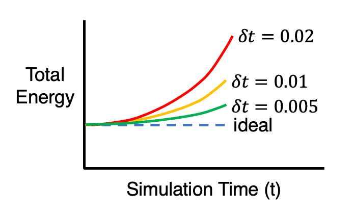
It should be emphasized that this sort of accuracy vs. computational time tradeoff is NOT unique to MD, and can be found in practically every computational modeling technique.

Code for MD spring demonstration and gif saving

current_positions = [-2,2] #positions of the particles
current_forces = [0,0] #starting forces on the particles
velocities = [0,0]
forces = [0,0]
mass = [1,1]

new_positions = [0,0]
new_forces = [0,0]

save_positions = []

iterations = 1000
timestep = 0.005


for i in range(iterations):

  #Save the current positions
  save_positions.append(current_positions.copy())

  #Update the positions
  for j in range(len(current_positions)):
    new_positions[j] = current_positions[j] + velocities[j]*timestep + (forces[j]/ (2*mass[j]) )*(timestep**2)


  #Find the total force on each particle
  for j in range(len(current_positions)):

    new_forces[j]=0

    for k in range(len(current_positions)):
      if j==k:
        continue

      distance = current_positions[j]-current_positions[k]
      sign = distance /abs(distance)

      new_forces[j] = new_forces[j]+10*(abs(distance)-5) * -sign

  #Update velocities
  for j in range(len(current_positions)):
    velocities[j] = velocities[j] + timestep*(forces[j] + new_forces[j])/(2*mass[j])

  #Set the force as the new forces
  for j in range(len(current_positions)):
    forces[j] = new_forces[j]

  #Set the new positions
  for j in range(len(current_positions)):
    current_positions[j]=new_positions[j]


#Plot the evolution of the particle position and create a gif

from matplotlib import pyplot as plt
from celluloid import Camera

fig = plt.figure()
plt.xlim([-4, 4])
plt.ylim([-1,1])
camera = Camera(fig)
for i in range(len(save_positions)):
    plt.scatter(save_positions[i],[0]*len(current_positions), s=120, c=[1]*len(current_positions))
    text = "T = " + str(round(timestep*i,2))
    plt.text(1, 0.5, text, ha='left',wrap=False)
    camera.snap()

animation = camera.animate()
animation.save('spring_gif.gif', writer = 'pillow', fps=40)

Thanks for reading!

References

1. Frenkel, Daan, and Berend Smit. Understanding Molecular Simulation from Algorithms to Applications. Academic Press, 2002.
2. Braun, Efrem, et al. “Best Practices for Foundations in Molecular Simulations [Article v1.0].” Living Journal of Computational Molecular Science, vol. 1, no. 1, 2019, doi:10.33011/livecoms.1.1.5957.