As usual, the full code can be found at the end of the article.
STEP 1 : Get the Satellite Orbit Data
In order to plot our satellite’s orbit, we first need to obtain the latest orbital data that open sources can provide. In the space sector, these information are known as “Ephemeris” and are usually provided once to twice a day for each orbiting object — satellites, rocket bodies, or even debries are monitored this way, all with their own identifier known as the NORAD id.
Ephemeris are delivered using the Two-Line Element set (or TLE) format, which informs about many orbital parameters such as the orbit shape, the satellite location on this orbit or the time at which the data was recorded, among others. As an exemple, here are the ISS latest Ephemeris’ TLE at the time I wrote these lines :
1 25544U 98067A   23308.63791865  .00019085  00000-0  34042-3 0  9990
2 25544  51.6442 352.8512 0001019  69.0284  39.5642 15.50096686423576
All this precious data will help us later reconstruct the full orbit with only two lines of 69 caracters in length ! Two great sources to gather these valuable ephemeris are Celestrak.org (which provides the latest Ephemeris’ TLE for a wide range of space objects) and space-track.org (provides the latest data AND allows for archive request of past ephemeris’ TLE).
For our case, we will use Celestrak, as it does not require any account creation, and will be sufficient for our needs. To obtain the data, go to the main page (here) and click on “search the SATCAT” among all the blue links. Note that SATCAT stands for satellite catalog, and is the standard name of any orbiting object listing in the space field.
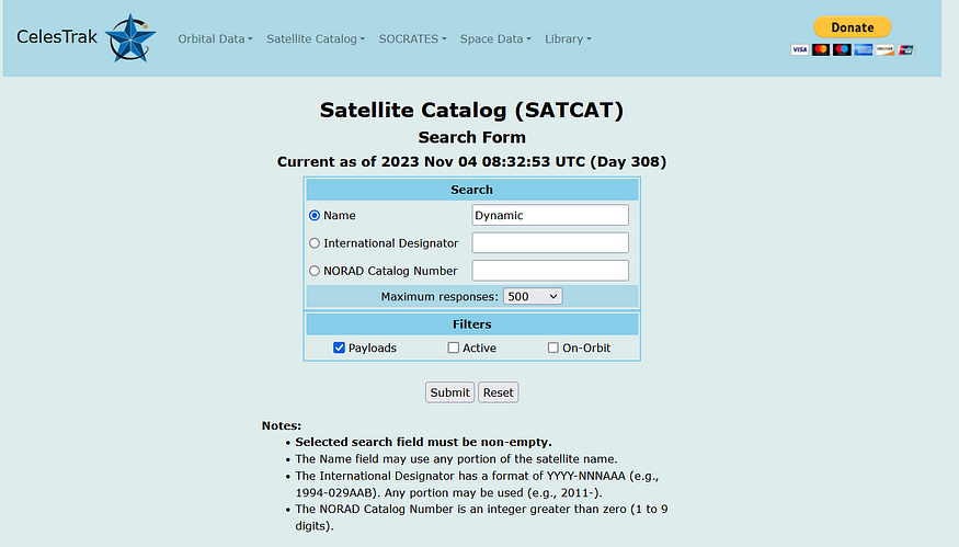
Once on the search page, you can look for any satellite you would like. Let’s take Dynamics Explorer 1 and Molniya ephemeris. As we will see later on, these satellites are following a rather elliptical orbit and the farther point from earth (the apogee, litterally “above-earth” in ancient greek) is a few tens of thousands of kilometers above ground, which will results in a nice plot.
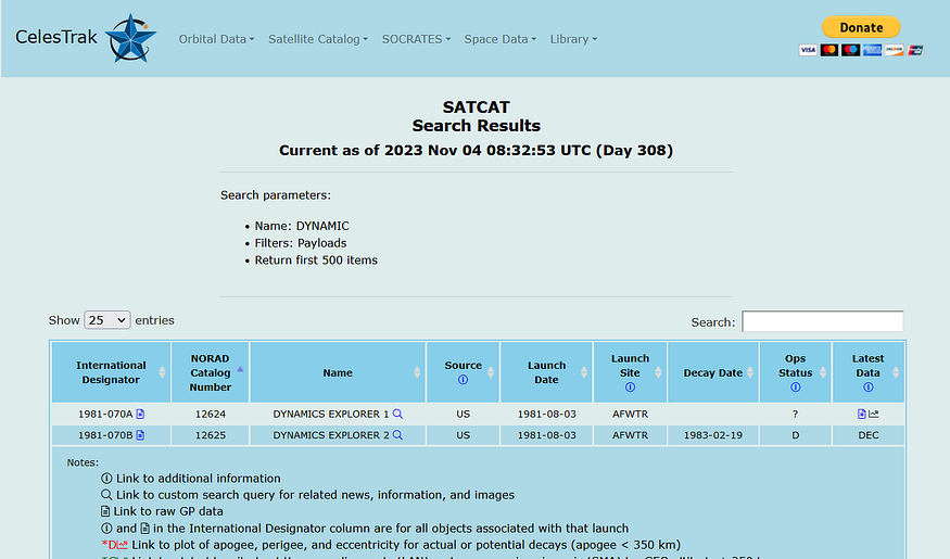
To get the data, simply click on the file icon at the end of the row. As you can also understand, the other satellite “Dynamics explorer 2” is not orbiting anymore, and thus no data can be provided. Here are the data at the time of redaction with the Dynamics explorer’s TLE in the first two rows and molniya TLE in the two last rows, yours should only slightly differ :
1 12624U 81070A   23308.22842017  .00000105  00000-0  62186-3 0  9995
2 12624  90.5880  39.8152 6226940 162.2035 237.0971  3.52681475691436
1 24960U 97054A   23308.28758058  .00000032  00000+0  71582-2 0  9994
2 24960  64.0340  48.8900 6106083 294.3666  15.0965  3.18688075224098
Once you get the data, you can freely add some other satellite’ TLE by appending the TLE, then copy and paste all the text as is into your notepad and save it as a .txt file, we’ll read it later with the help of python.
STEP 2 : Get the Python Script Ready
As usual, we will import the necessary libraries for our work. For this task, we will use math and numpy to deal with the orbital equations and rotations in the plot, datetime to get a usable time format from the TLE and, as expected, matplotlib will be used to plot our orbit.
import matplotlib.pyplot as plt
import numpy as np
import datetime as dt
import math as m
STEP 3 : Read the Data
From the file that we saved earlier on, we will read the useful data and save it in a dictionnary named orb with a direct access to orbital parameters. I also define three constants that will come handy for the orbital computation : mu is earth’s standard gravitational parameter, r is earth’s radius and D is the amount of hours in a sideral day.
#Put your own file path here
ADDR = "C:\\Users\\username\\Documents\\Secret_folder\\tle.txt"
TLE = open(ADDR,"r").readlines()

#CHANGE THESE VALUES IF YOU ARE NOT ORBITING EARTH !
mu = 398600.4418
r = 6781
D = 24*0.997269
We will then parse the data from the file, without going through details, we simply read the TLE numbers and give them meaning in the python dictionary orb. In order to read many TLE in a single file and to be able to re-use the code, we’ll put that in a function and in a for loop, looping through the file’s lines:
def plot_tle(data):
    fig = plt.figure()
    ax = plt.axes(projection='3d',computed_zorder=False)
    for i in range(len(data)//2):
        if data[i*2][0] != "1":
            print("Wrong TLE format at line "+str(i*2)+". Lines ignored.")
            continue
        if int(data[i*2][18:20]) > int(dt.date.today().year%100):
            orb = {"t":dt.datetime.strptime("19"+data[i*2][18:20]+" "+data[i*2][20:23]+" "+str(int(24*float(data[i*2][23:33])//1))+" "+str(int(((24*float(data[i*2][23:33])%1)*60)//1))+" "+str(int((((24*float(data[i*2][23:33])%1)*60)%1)//1)), "%Y %j %H %M %S")}
        else:
            orb = {"t":dt.datetime.strptime("20"+data[i*2][18:20]+" "+data[i*2][20:23]+" "+str(int(24*float(data[i*2][23:33])//1))+" "+str(int(((24*float(data[i*2][23:33])%1)*60)//1))+" "+str(int((((24*float(data[i*2][23:33])%1)*60)%1)//1)), "%Y %j %H %M %S")}
        orb.update({"name":data[i*2+1][2:7],"e":float("."+data[i*2+1][26:34]),"a":(mu/((2*m.pi*float(data[i*2+1][52:63])/(D*3600))**2))**(1./3),"i":float(data[i*2+1][9:17])*m.pi/180,"RAAN":float(data[i*2+1][17:26])*m.pi/180,"omega":float(data[i*2+1][34:43])*m.pi/180})
        orb.update({"b":orb["a"]*m.sqrt(1-orb["e"]**2),"c":orb["a"]*orb["e"]})
STEP 4 : Get the orbits right
In order to remain accessible to every reader, I will not dive too deep within the maths behind the next lines, but here is what you need to know in a nutshell :
An orbit’s shape can be simply defined by two values :
- its excentricity : the “e” value in the data — exactly 0 and the orbit is perfectly circular, from 0.1 to 0.9 the orbit gets more and more elliptical, above 1 and the object is escaping earth’s gravity with an hyperbola trajectory
- its semi-major axis : the “a” value in the data — it is the length of the longest “radius” you can find in an ellipse. One can also understand it as the size factor of the ellipse defined previously with the excentricity: a large semi-major axis gives a large orbit far from its attracting body.
Then, once you get the shape right, it is just a matter of rotating that shape so that it orbits the earth in the good plane, and then placing earth in one of the orbit’s focus. We have thus three rotations to perform :
- firts we rotate the orbit along the z-axis in the equatorial plane to match the points where it crosses the celestial equator (an extension in space of our beloved equatorial line) with the RAAN,
- then we rotate the orbit out of the celestial equatorial plane along that new x axis we rotated previously, with the inclination (0° gives an equatorial orbit, +90° or -90° gives a polar orbit),
- and finally, we rotate the orbit itself in its own new plane we’ve defined with the previous rotations to put the perigee (closest point of an orbit from the earth, litterally “around earth” in ancient greek) at the right spot with the omega value (also called argument of perigee).

orbit rotations (form right to left)
All these steps are summarized in a few lines of code where we build a rotation matrix R to perform these rotations on the ellipse’s parametric equation values (please click the underlined links if you want to know more). We then store the x, y and z values to plot them in the next section.
# R is our rotation matrix built from three rotations
R = np.matmul(np.array([[m.cos(orb["RAAN"]),-m.sin(orb["RAAN"]),0],[m.sin(orb["RAAN"]),m.cos(orb["RAAN"]),0],[0,0,1]]),(np.array([[1,0,0],[0,m.cos(orb["i"]),-m.sin(orb["i"])],[0,m.sin(orb["i"]),m.cos(orb["i"])]])))
R = np.matmul(R,np.array([[m.cos(orb["omega"]),-m.sin(orb["omega"]),0],[m.sin(orb["omega"]),m.cos(orb["omega"]),0],[0,0,1]]))
x,y,z = [],[],[]
# we loop through the parametric orbit and compute the positions' x, y, z
for i in np.linspace(0,2*m.pi,100):
    P = np.matmul(R,np.array([[orb["a"]*m.cos(i)],[orb["b"]*m.sin(i)],[0]]))-np.matmul(R,np.array([[orb["c"]],[0],[0]]))
    x += [P[0]]
    y += [P[1]]
    z += [P[2]]
STEP 5 : Time to Plot !
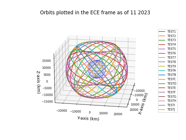
Finally, we can give a meaning to all this extracted data by showing the orbits around a blue wireframe sphere which will be our earth planet. The orbits are identified by their NORAD number.
    #we plot the orbits in the for loop
    ax.plot(x,y,z,zorder=5)
#then we plot the earth
u, v = np.mgrid[0:2*np.pi:20j, 0:np.pi:10j]
ax.plot_wireframe(r*np.cos(u)*np.sin(v),r*np.sin(u)*np.sin(v),r*np.cos(v),color="b",alpha=0.5,lw=0.5,zorder=0)
plt.title("Orbits plotted in the ECE frame as of "+orb["t"].strftime("%m %Y"))
ax.set_xlabel("X-axis (km)")
ax.set_ylabel("Y-axis (km)")
ax.set_zlabel("Z-axis (km)")
ax.xaxis.set_tick_params(labelsize=7)
ax.yaxis.set_tick_params(labelsize=7)
ax.zaxis.set_tick_params(labelsize=7)
ax.set_aspect('equal', adjustable='box')
if len(data)//2 < 5:
    ax.legend()
else:
    fig.subplots_adjust(right=0.8)
    ax.legend(loc='center left', bbox_to_anchor=(1.07, 0.5), fontsize=7)
plt.show()
STEP 6 : Enjoy !
From this code, we can now print our orbits easily in only three lines of code for as many TLE as we’d like !
ADDR = "C:\\Users\\username\\Documents\\Secret_folder\\tle.txt"
TLE = open(ADDR,"r").readlines()
plot_tle(TLE)

STEP 7 : Plot some more with modified TLEs !
Congrats, you made it until the end ! Here are a few examples of what this piece of code can do, with modified TLE to get some interesting orbits.


Thanks for reading ! If you need to quickly get the code, here it is in its entirety :
import matplotlib.pyplot as plt
import numpy as np
import datetime as dt
import math as m

mu = 398600.4418
r = 6781
D = 24*0.997269

def plot_tle(data):
    fig = plt.figure()
    ax = plt.axes(projection='3d',computed_zorder=False)
    for i in range(len(data)//2):
        if data[i*2][0] != "1":
            print("Wrong TLE format at line "+str(i*2)+". Lines ignored.")
            continue
        if int(data[i*2][18:20]) > int(dt.date.today().year%100):
            orb = {"t":dt.datetime.strptime("19"+data[i*2][18:20]+" "+data[i*2][20:23]+" "+str(int(24*float(data[i*2][23:33])//1))+" "+str(int(((24*float(data[i*2][23:33])%1)*60)//1))+" "+str(int((((24*float(data[i*2][23:33])%1)*60)%1)//1)), "%Y %j %H %M %S")}
        else:
            orb = {"t":dt.datetime.strptime("20"+data[i*2][18:20]+" "+data[i*2][20:23]+" "+str(int(24*float(data[i*2][23:33])//1))+" "+str(int(((24*float(data[i*2][23:33])%1)*60)//1))+" "+str(int((((24*float(data[i*2][23:33])%1)*60)%1)//1)), "%Y %j %H %M %S")}
        orb.update({"name":data[i*2+1][2:7],"e":float("."+data[i*2+1][26:34]),"a":(mu/((2*m.pi*float(data[i*2+1][52:63])/(D*3600))**2))**(1./3),"i":float(data[i*2+1][9:17])*m.pi/180,"RAAN":float(data[i*2+1][17:26])*m.pi/180,"omega":float(data[i*2+1][34:43])*m.pi/180})
        orb.update({"b":orb["a"]*m.sqrt(1-orb["e"]**2),"c":orb["a"]*orb["e"]})
        R = np.matmul(np.array([[m.cos(orb["RAAN"]),-m.sin(orb["RAAN"]),0],[m.sin(orb["RAAN"]),m.cos(orb["RAAN"]),0],[0,0,1]]),(np.array([[1,0,0],[0,m.cos(orb["i"]),-m.sin(orb["i"])],[0,m.sin(orb["i"]),m.cos(orb["i"])]])))
        R = np.matmul(R,np.array([[m.cos(orb["omega"]),-m.sin(orb["omega"]),0],[m.sin(orb["omega"]),m.cos(orb["omega"]),0],[0,0,1]]))
        x,y,z = [],[],[]
        for i in np.linspace(0,2*m.pi,100):
            P = np.matmul(R,np.array([[orb["a"]*m.cos(i)],[orb["b"]*m.sin(i)],[0]]))-np.matmul(R,np.array([[orb["c"]],[0],[0]]))
            x += [P[0]]
            y += [P[1]]
            z += [P[2]]
        ax.plot(x,y,z,zorder=5,label=orb["name"])
    u, v = np.mgrid[0:2*np.pi:20j, 0:np.pi:10j]
    ax.plot_wireframe(r*np.cos(u)*np.sin(v),r*np.sin(u)*np.sin(v),r*np.cos(v),color="b",alpha=0.5,lw=0.5,zorder=0)
    plt.title("Orbits plotted in the ECE frame as of "+orb["t"].strftime("%m %Y"))
    ax.set_xlabel("X-axis (km)")
    ax.set_ylabel("Y-axis (km)")
    ax.set_zlabel("Z-axis (km)")
    ax.xaxis.set_tick_params(labelsize=7)
    ax.yaxis.set_tick_params(labelsize=7)
    ax.zaxis.set_tick_params(labelsize=7)
    ax.set_aspect('equal', adjustable='box')
    if len(data)//2 < 5:
        ax.legend()
    else:
        fig.subplots_adjust(right=0.8)
        ax.legend(loc='center left', bbox_to_anchor=(1.07, 0.5), fontsize=7)
    plt.show()

ADDR = "C:\\Users\\username\\Documents\\Secret_folder\\tle.txt"
TLE = open(ADDR,"r").readlines()
plot_tle(TLE)
Comments
Loading comments…