Cross-Validation Explained
Cross-validation is a method that can estimate the performance of a model with less variance than a single ‘train-test' set split. It works by splitting the dataset into k-parts (i.e. k = 5, k = 10). Each time we split the data, we refer to the action as creating a ‘fold'. The model is trained on k-1 folds with one held back and tested on the held back part. Each fold should be as close to the same record size as possible. After running cross-validation, you end up with k different performance scores that we summarize using the mean and standard deviation.
Assume we have a dataset (n=5,000 records total) split into k = 5 parts (each part n = 1,000). We label the parts A, B, C, D, and E. The model would be trained 5 times. Each time, 4 (K-1) folds would be included in the training group and the 5th fold would be the testing group. The testing group rotates each time the model is trained. An example of a k = 5 cross-validation model follows:
- Training 1: Training folds = A, B, C, D while E is the testing fold
- Training 2: Training folds = B, C, D, E while A is the testing fold
- Training 3: Training folds = C, D, E, A while B is the testing fold
- Training 4: Training folds = D, E, A, B while C is the testing fold
- Training 5: Training folds = E, A, B, C while D is the testing fold
The result is a more reliable estimate of the performance of the model on new data. It is more accurate because the model is trained and evaluated multiple times on different data. The choice of k must allow the size of each test partition to be large enough to be a reasonable sample of the problem while allowing enough repetitions of the ‘train-test' evaluation to provide a fair estimate of the model's performance on unseen data. For many datasets with thousands or tens of thousands of records, k values of 3, 5, and 10 are common.
A Python Step-by-Step Walkthrough
# Load the required libraries
import numpy as np
import pandas as pd
from sklearn.model_selection import KFold
from sklearn.model_selection import cross_val_score
from sklearn.linear_model import LogisticRegression
from sklearn.metrics import confusion_matrix
from sklearn.metrics import classification_report
The original dataset is on www.ibm.com.
# Load the data file. Add the correct directory path to reach the
# file on your computer or network.
df=pd.read_csv(r'WA_Fn-UseC_-Telco-Customer-Churn.csv')
The file is loaded and placed into a dataframe. When it's reasonably possible, I like to see all of my columns. I set the display to show all columns and output the 5-row head to see how the column titles and first few rows of data look.
# Organize dataframe. Display the first five rows and column titles.pd.set_option('display.max_columns', None) # Display all columns
df.head()

Data Cleaning
Next, I want to make sure the numerical data is in a usable format (integer or float).
df.columns.values

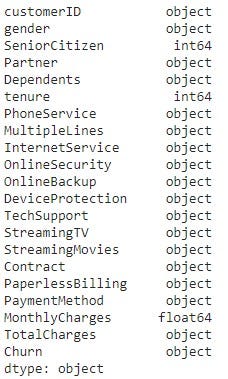
df.dtypes

Fortunately, we did not overlook this step. We discover the TotalCharges column appears as an object. It has to be an integer for us to work with it. We can fix this by converting it to numeric. Also, at this time, I will look for missing values.
# Converting Total Charges to a numerical data type. Currently in dataframe as an object.
df.TotalCharges = pd.to_numeric(df.TotalCharges, errors='coerce')
df.isnull().sum()  # Count the number of missing values

We coerce the TotalCharges column to numerical and then determine the only missing data are 11 items in the TotalCharges column. 11 is minimal, so I decide to delete those observations from the dataset. Since customer ID has no purpose other than to identify who the data belongs to, we eliminate that column from the dataset.
Next, in this code block, we need to convert our response and predictor variables into usable formats. Churn is our response variable and we will convert it from an object to an integer. We assign each yes = 1 and no = 0. Finally, we have to convert the categorical predictor variables into (numerical) dummy variables. Then we take another look at the header.
# Removing missing values
df.dropna(inplace = True)
# Remove customer IDs from the data set
df2 = df.iloc[:,1:]
# Converting the predictor variable into a binary numeric variable
df2['Churn'].replace(to_replace='Yes', value=1, inplace=True)
df2['Churn'].replace(to_replace='No',  value=0, inplace=True)
# Convert all the categorical variables into dummy variables
df_dummies = pd.get_dummies(df2)
df_dummies.head()

This header looks much different from the previous one. All the objects have been converted to 0's and 1's. The data is now ready for logistic regression.
Logistic Regression
The first step in logistic regression is to assign our response (Y) and predictor (x) variables. In this model, Churn is our only response variable and all the remaining variables will be predictor variables.
# assign X to all the independent (predictor) variables, assign Y to the dependent (response) variable
X = df_dummies[['SeniorCitizen','tenure','MonthlyCharges','TotalCharges','gender_Female','gender_Male','Partner_No','Partner_Yes','Dependents_No','Dependents_Yes','PhoneService_No','PhoneService_Yes','MultipleLines_No','MultipleLines_No phone service','MultipleLines_Yes','InternetService_DSL','InternetService_Fiber optic','InternetService_No','OnlineSecurity_No','OnlineSecurity_No internet service','OnlineSecurity_Yes','OnlineBackup_No','OnlineBackup_No internet service','OnlineBackup_Yes','DeviceProtection_No','DeviceProtection_No internet service','DeviceProtection_Yes','TechSupport_No','TechSupport_No internet service','TechSupport_Yes','StreamingTV_No','StreamingTV_No internet service','StreamingTV_Yes','StreamingMovies_No','StreamingMovies_No internet service','StreamingMovies_Yes','Contract_Month-to-month','Contract_One year','Contract_Two year','PaperlessBilling_No','PaperlessBilling_Yes','PaymentMethod_Bank transfer (automatic)','PaymentMethod_Credit card (automatic)','PaymentMethod_Electronic check','PaymentMethod_Mailed check' ]]

Y = df_dummies['Churn']
This is followed by running the k-fold cross-validation logistic regression.
# 5 folds selected
kfold = KFold(n_splits=5, random_state=0, shuffle=True)
model = LogisticRegression(solver='liblinear')
results = cross_val_score(model, X, Y, cv=kfold)
# Output the accuracy. Calculate the mean and std across all folds.
print("Accuracy: %.3f%% (%.3f%%)" % (results.mean()*100.0, results.std()*100.0))

This refers to classification accuracy, which is the number of correct predictions as a percentage of all predictions made. Our model has produced an accuracy of 80.333% (mean) with a standard deviation of 1.080%. When looking at the underlying dataset, I found the company had approximately 26% of its customers leave each period, while the 74% remained as customers (this was provided as a note accompanying the data file).
Besides specifying the size of the split (k=5), we also specify a random seed (random_state=0). Because the split of the data is random, we want to ensure the results are reproducible. By specifying the random seed, we ensure we get the same random numbers each time we run the code and in turn the same split of data. This is important if we want to compare this result to the estimated accuracy of another model. To ensure the comparison was apples-for-apples, we must ensure they are trained and tested on exactly the same data.
Interpretation of Model Output
Accuracy is best when the number of observations in each class is the same. There are approximately 3 times as many customers retained as those who leave, so accuracy may not be the best way to view our answer. Since we like statistics, let's dig a little deeper to get a few more meaningful numbers with a different model. It's time to create a confusion matrix using a training size = .67 with a test size = .33 on the same dataset.
# Construct a confusion matrix
test_size = 0.33
seed = 0
X_train, X_test, Y_train, Y_test = train_test_split(X, Y, test_size=test_size,
random_state=seed)
model = LogisticRegression(solver='liblinear')
model.fit(X_train, Y_train)
predicted = model.predict(X_test)
matrix = confusion_matrix(Y_test, predicted)
print(matrix)

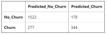
A confusion matrix (screenshot above) may be one of the least insightful visuals in the entire python language. Luckily, there is a way to make it more meaningful.
#transform confusion matrix into array
#the matrix is stored in a vaiable called confmtrx
confmtrx = np.array(matrix)
#Create DataFrame from confmtrx array
#rows for test: Churn, No_Churn designation as index
#columns for preds: Pred_Churn, Pred_NoChurn as columnpd.DataFrame(confmtrx, index=['No_Churn','Churn'],
columns=['Predicted_No_Churn', 'Predicted_Churn', ])

That is much better. This chart allows us to more clearly understand the quadrants. We see the model predicted “no churn” 1,799 times (1,522 + 277). It was correct 1,522 times and incorrect 277 times (85% correct) when it predicted “no churn”. The model predicted “churn” 522 times (178 + 344). It was correct 344 of those times and incorrect 178 times (66% correct) when “churn” was predicted. Now, besides 80%, we have 85% and 66%. Which is correct? Fortunately, we can create a classification report to help us sort everything out.
# Create a classification report. Use the same test size and same
# seed number before.
test_size = 0.33
seed = 0
X_train, X_test, Y_train, Y_test = train_test_split(X, Y, test_size=test_size,
random_state=seed)
model = LogisticRegression(solver='liblinear')
model.fit(X_train, Y_train)
predicted = model.predict(X_test)
report = classification_report(Y_test, predicted)
print(report)

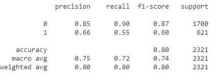
The screenshot above shows a classification report. There are four statistical columns: precision, recall, f1-score, and support. Precision refers to what percent of our predictions were correct. This is where the 85% and 66% originated. The macro average is calculated as(.85 + .66)/2. The model uses greater precision than two decimal places and rounds at two decimal places. Finally, we arrive at .80 = (1700/2321).85 + (621/2321).66.
Recall is the percentage of positive (or negative) cases the model could detect. In this scenario (1,522/1,700) = .90 and (344/621)=.55. The macro average and weighted average are computed using the same methods shown for precision.
The F1-score is a weighted harmonic mean of precision and recall where the best possible score is 1.0 and the worst possible score is 0.0. It is considered better to use the weighted average of the F1 score to compare models, not the global accuracy score. In this model, both are 0.80, so there is no difference between the global accuracy and the weighted F1-score.
The support column provides the user with the number of observations in each row and column.
Summary
The model using k-fold cross-validation (k=5) reported accuracy of 80.333% with a standard deviation of 1.080%. The confusion matrix/classification report model reported a weighted average F1 score = 80% and a global accuracy score = 80%. The k-fold cross-validation model was almost identical to the results of the confusion matrix/classification report model.
Please give this k-fold cross-validation a try and let me know if you have questions or run into an issue.
Comments
Loading comments…