I have previously written on the potential use of unsupervised machine learning to classify football players. Given a set of forwards playing in the French top flight last season (22/23), I used the k-means clustering method to identify 3 types of forward. The algorithm grouped players like Kylian Mbappe, Neymar and Alexis Sanchez in one cluster. Wissam Ben Yedder, Terem Moffi and Lois Openda can be found among the players in the second cluster. Sofiane Boufal, Dimitri Payet (remember him?) and Desire Doue are some of whom who are assigned to the third and final cluster. For a comprehensive exploration of the cluster characteristics, read the original post here.

The aim of this post is to build upon the aforesaid premise, I will use unsupervised machine learning to identify similar players with a more refined approach and expand my search to forwards across Europe's big 5 leagues.

As the use of analytics in sport continues to expand, football in particular, there has been a significant increase in the use of complex models to analyse aspects related to the game. While a lot of these models are built under the supervised framework, the following takes up for the continued use of unsupervised techniques in football. To skip the explanation of the methods used, scroll down to the Methods section.

K-means:

The most common unsupervised technique is probably clustering. And in this paradigm, the aforementioned k-means is this most popular. A comprehensive breakdown of the method is as follows:

1. The practitioner must first specify some 'K' value which determines the number of clusters in the algorithm's output
2. Then, initialise 'K' random vectors in R^n where n is the number of features in the dataset. These are referred to as the initial cluster centroids
3. The k-means objective function measures the squared distance between each data point to each of the centroids: assignment rules are based on the closest centroid, different distance calculations can be used such as Euclidean, Manhattan (Shutaywi, 2021)
4. After assignment, the centroid is updated and moved to the mean of all data points in that cluster
5. This iterative process is repeated until convergence: when the cluster centers move very little or not at all (Hartigan et al., 1979)

The algorithm aims to find underlying patterns in the data distribution and it's output is groups (clusters) of samples (players) that are sufficiently close to each other in R^n where n is the number of features. It's application in sport can easily be seen: clustering can be used by recruitment departments to identify replacements for departing players or suitable alternatives to transfer targets. It extends beyond player level and can be used to profile team profiles (Spencer et al., 2016), identify missing player profiles and potentially evaluate the optimal team composition based on player profiles. Overall, the method is computationally efficient and can handle large datasets all while producing clusters that are easy to interpret and can be used for further analysis or decision-making (Bishop, 2006). This provides credence for it's use in clustering the Ligue 1 forwards previously.

Drawbacks:

However, as with anything, k-means has its pitfalls. Notably, the clustering outcomes hinge on the proper selection of the hyperparameter 'K', which represents the number of clusters. However, determining the optimal 'K' is often a non-trivial task and is seldom known beforehand. This predicament requires end users to possess domain knowledge, violating the reliability condition in valid statistical analysis (Kodinariya et al., 2013). The assumption that users have prior insights into the dataset's structure may introduce subjectivity and compromise the objectivity of the clustering process.

K-means clustering also performs hard clustering. It maintains a 1:1 ratio between points and clusters: each point is assigned exclusively to one cluster. This strict assignment may lead to some loss of information as the algorithm assumes that each point can only belong to one cluster. More realistically, some data points may exhibit similarities with multiple clusters or may not perfectly fit into any cluster at all. When used in a football context, it is obvious that this can be problematic. Different players may be a hybrid of two types but the model outputs do not account for this.

Consider the findings from Kumar et al. (2019) who used k-means to discover that different types of athletes face different pressures due to their own conditions and external environment, and their stressors are quite different. It is both plausible and likely that there are athletes who face the same pressures as those in their assigned cluster but to a different degree. Referring back to the clustering of team profiles in the AFL, it is very likely that there are teams exhibiting playing styles that resemble multiple clusters depending on opponent or manager. This restrictive assumption has given rise to other clustering methods such as fuzzy clustering (Bezdek, 2013).

Gaussian Mixed Models:

One method of fuzzy clustering is the use of Gaussian Mixed Models (GMMs). These are probabilistic models that represent a blend of multiple Gaussian distributions. Each distribution corresponds to a cluster in the data. An amalgamation of normal distributions that can be separated by the probability of each data sample belonging to a particular cluster. The model parameters are found by Expectation-Maximisation Algorithms. A deeper (and better) explanation of GMMs and Expectation-Maximisation can be found here.

To justify the use of a GMM in this case, it is helpful to state an assumption in k-means: k-means algorithms assume that clusters are spherical and equally sized (Saskia et al., 2006). Given a dataset of all of the forwards in Europe's big 5 leagues, this could prove to be a costly assumption.

Another benefit of using a GMM is the soft clustering. The model outputs the probabilities of each player belonging to each group, providing insight into which players can potentially operate in multiple roles. The probabilities also make us privy to the strength of the perceived similarity of a specific player to his assigned cluster.

The use of probabilities can also be seen as a method of evaluating the cluster assignments. Consider a GMM with 3 components, the probability that a single player belongs to each of the clusters must equal 1. A model that outputs probabilities close or equal to 1 for most players provides confidence that the specified number of components is close to optimal.

Overall, a GMM is better suited to cases with complex data distributions where clusters may have different shapes or sizes. A caveat however, is that similarly to k-means, the number of components (clusters) needs to be specified beforehand. A hybrid approach that uses k-means to find the optimal number of components and GMM to produce clusters has been used in machine learning (Jebrani, 2021) and will be used here.

Method:

This section details how I used a hybrid method in Python to classify forwards across Europe. The full code is provided in the appendix.

It should be noted that I used the k-medoids technique as opposed to k-means to find the optimal 'K'. In k-medoids, representative objects known as medoids replace centroids, and the method is less susceptible to outliers due to its reliance on the most centrally located object in a cluster (Park et al., 2009).

The k-means algorithm is sensitive to outliers. In the random initialisation, if outliers are used as an initial centroid then the algorithm's efficiency will be reduced. Cluster centroids that aren't outliers may also be dragged by outliers. As the algorithm is easily influenced by noise and outliers, the clustering results may be unsatisfactory (Chong, 2021). Despite the higher complexity of the k-medoids algorithm, studies have shown its superior performance in terms of execution time, non-sensitivity to outliers, and noise reduction (Arora et al., 2016).

1. Webscraping

The first step required me to scrape the necessary data from FBREF, and store the data in Pandas dataframes. Data cleaning is required to combine dataframes, remove duplicate columns and rename ambigiously named columns.

2. Data Filtering

Next, I filtered my cleaned dataframe to forwards ("FW") and those who have played more than the median number of minutes at this stage of the season. This helps to mitigate spurious effects in the data and improve model results.

3. Feature Engineering

Feature selection is next. To gain a true impression of a player's habits and tendencies, only action-based features were selected whilst outcome features were abandoned. Features included measures such as pass volume, shot volume, tackles and shots whilst outcome features such as expected goals, pass completion and expected assists are abandoned. This is level the playing field between those playing in top teams and those in struggling teams.

The features were also normalised at this stage between 1 and 10. This is important as we would like all features to be equally weighted. This step ensures that no individual feature dominates the distance calculated by the algorithm.

The final set of features are:

['player', 'pos', 'squad', 'comp', 'age', '90s', 'min', 'shots', 'shots on target',
'shot dist', 'total pass att', 'short pass att', 'med pass att', 'long pass att', 'passes into the penalty area', 'crosses into the penalty area', 'progressive passes', 'through balls', 'total tackles', 'tackles defensive 3rd', 'tackles mid 3rd', 'tackles att 3rd', 'blocks', 'interceptions', 'clearances', 'errors', 'touches', 'touches def pen', 'touches def 3rd', 'touches mid 3rd', 'touches att 3rd', 'touches att pen', 'carries', 'progressive carries']

4. K-medoids

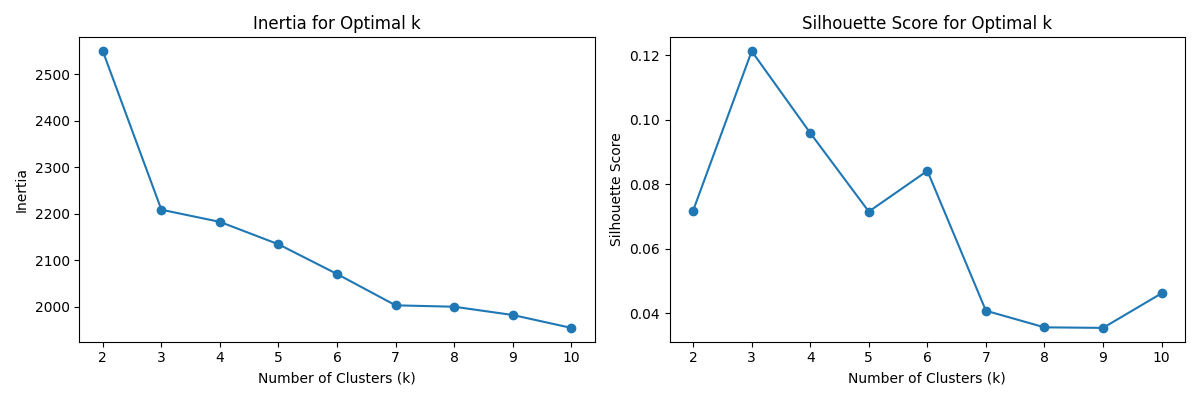
A k-medoids algorithm is fitted to the features and both the Silhouette score and Elbow method are used to identify the optimal K clusters. The concensus is 3. The results are visualised below:

5. GMM

Finally, a GMM is fitted to our dataset setting the parameter ncomponent = 3. Using the scikit-learn Python library, we are able to obtain the cluster means (gmm.means), cluster weights (gmm.weights*) and cluster covariances (gmm.covariances*).

gmm.means: this returns an array where the rows are each individual cluster and the columns are the mean value of each input feature for that cluster

gmm.weights: this returns an array representing the weights of the individual components, each weight corresponds to the contribution of each component to the overall mixture. Weights are the sum of the probabilities of each of their samples belonging to the respective cluster. Component weights sum to 1 thereby, a weight of 0.6 implies that a component contributes 60% to the overall mixture.

gmm.covariances: this returns a list of arrays detailing the covariance matrices of each component. The covariances* attribute provides information about the spread and orientation of the Gaussian distributions in each cluster. This helps us to grasp the shape of each cluster and the correlation between features within each cluster.

6. Model Output

To convey the algorithm's output, I have randomly selected 5 players from each cluster,

Cluster 1: Bukayo Saka, Mohammed Salah, Khvicha Kvaratskhelia, Antoine Griezmann, Rayan Cherki

Cluster 2: Michail Antonio, Antony, Pierre-Emerick Aubameyang, Taiwo Awoniyi, Folarin Balogun

Cluster 3: Matheus Cunha, Jeremy Doku, Vinicius Júnior, Takefusa Kubo, Rafael Leão

For some intuition, we can compare the distribution of players output for a specific metric, below we can see the distribution of total player touches for each cluster. The second component recorded the highest weight (73%) and this is seen in the graph. Players in the second component average the lowest number of touches, around 250 per game relative to the other clusters and this is consistent with domain knowledge. Forwards such as Antonio, Aubameyang and Awoniyi are traditional *number 9's *who tend not to get too involved in build-up and generally play close to the last line of defense.

Conclusion

Further analysis can be gleamed from the model's output. What is the distribution across the different leagues? Which players could potentially be assigned to multiple clusters? And so on.

This method could be improved: further feature engineering to adjust metrics by possession to further mitigate the impact of team quality on player statistics. It may also be more informative to look at player stats on a per game basis instead of absolutely.

To close, I hope this piece has convinced you of the utility of unsupervised learning in football. Whilst results should not be used as the sole source of truth for decision making, this can supplement the decision making process and also provide a platform for further analysis.

If you've made it this far, any and all scrutiny is not only welcome but encouraged. For contact, email me: remiawosanya8@gmail.com

Appendix:

Code:

Libraries

import requests
from bs4 import BeautifulSoup
import pandas as pd
import time
import matplotlib.pyplot as plt
import seaborn as sns
from sklearn_extra.cluster import KMedoids
from sklearn.metrics import silhouette_score
import numpy as np
from sklearn.mixture import GaussianMixture
import seaborn as sns

# Scrape Data

#region ----------------------------------------- #
main_page = "https://fbref.com/en/comps/Big5/stats/players/Big-5-European-Leagues-Stats"

def get_table_url(url):
 data = requests.get(url)
 soup = BeautifulSoup(data.text, "lxml")
 section = soup.select("div.section_wrapper")[0]
 links = [f"https://fbref.com{l.get('href')}" for l in section.find_all("a") if "/players/" in l.get('href')]
 return links

def get_player_stats(url_index, match_phrase, rename_dict):
 urls = get_table_url(main_page)
 data = requests.get(urls[url_index])
 df = pd.read_html(data.text, match=match_phrase)[0]
 df.columns = df.columns.droplevel()
 df.reset_index(drop=True, inplace=True)
 df.columns = [x.lower() for x in df.columns]

    # drop table divider rows
    df = df.loc[df["rk"] != "Rk"]
    df = df.drop("pos", axis=1).join(df["pos"].str.split(",", expand=True).stack().reset_index(drop=True, level=1).rename("pos"))
    df.columns = df.columns.str.strip()
    df = df.apply(lambda x: pd.to_numeric(x, errors='ignore'))

    cols = pd.Series(df.columns)
    duplicate_columns = cols[cols.duplicated()].unique()

    for dup in duplicate_columns:
        cols[cols[cols == dup].index.values.tolist()] = [f"{dup}.{i}" if i != 0 else dup for i in range(sum(cols == dup))]
    df.columns = cols

    if rename_dict:
        df.rename(columns=rename_dict, inplace=True)

    time.sleep(1)
    return df

player_summary_stats = get_player_stats(0, "Player Standard Stats", {
 "gls.1": "gls/90",
 "ast.1": "ast/90",
 "g+a.1": "g+a/90",
 "g-pk.1": "g-pk/90",
 "g+a-pk": "g+a-pk/90",
 "xg.1": "xg/90",
 "xag.1": "xag/90",
 "xg+xag": "xg+xag/90",
 "npxg.1": "npxg/90",
 "npxg+xag.1": "npxg+xag/90"
})

player_shooting_stats = get_player_stats(3, "Player Shooting", None)

player_passing_stats = get_player_stats(4, "Player Passing", {
 "cmp": "total_cmp",
 "att": "total_att",
 "cmp%": "total_cmp_pct",
 "cmp.1": "short_cmp",
 "att.1": "short_att",
 "cmp%.1": "short_cmp_pct",
 "cmp.2": "med_cmp",
 "att.2": "med_att",
 "cmp%.2": "med_cmp_pct",
 "cmp.3": "long_cmp",
 "att.3": "long_att",
 "cmp%.3": "long_cmp_pct"
})

player_passtypes_stats = get_player_stats(5, "Player Pass Types", None)

player_gca_stats = get_player_stats(6, "Player Goal and Shot Creation", {
 "passlive": "sca_passlive",
 "passdead": "sca_passdead",
 "to": "sca_takeons",
 "sh": "sca_shots",
 "fld": "sca_fld",
 "def": "sca_def",
 "passlive.1": "gca_passlive",
 "passdead.1": "gca_passdead",
 "to.1": "gca_takeons",
 "sh.1": "gca_shots",
 "fld.1": "gca_fld",
 "def.1": "gca_def"
})

player_def_stats = get_player_stats(7, "Player Defensive Actions", {
 "tkl": "total_tkl",
 "tkl.1": "drib_tkld",
 "att": "tkl_att",
 "def 3rd": "tkl_def_3rd",
 "mid 3rd": "tkl_mid_3rd",
 "att 3rd": "tkl_att_3rd",
 "past": "drib_past",
 "sh": "shots_blocked",
 "pass": "pass_blocked"
})

player_poss_stats = get_player_stats(8, "Player Possession", None)

player_summary_stats = player_summary_stats[["player", "pos", "squad", "comp", "age", "90s", "min"]]
player_shooting_stats = player_shooting_stats[["sh", "sot", "dist"]]
player_passing_stats = player_passing_stats[["total_att", "short_att", "med_att", "long_att", "ppa",
                                             "crspa", "prgp"]]
player_passtypes_stats = player_passtypes_stats[["tb"]]
player_def_stats = player_def_stats[["total_tkl", "tkl_def_3rd", "tkl_mid_3rd", "tkl_att_3rd",
                                     "blocks", "int", "clr", "err"]]
player_poss_stats = player_poss_stats[["touches", "def pen", "def 3rd", "mid 3rd", "att 3rd", "att pen",
                                       "carries", "prgc"]]

joint_df = pd.concat([player_summary_stats, player_shooting_stats, player_passing_stats, player_passtypes_stats,
 player_def_stats, player_poss_stats], axis=1).reset_index(drop=True)
#endregion ---------------------------------------- #

# Data Filtering

#region ----------------------------------------- #
def data_processing(pos):
 med_mins = joint_df["min"].median()
 filtered_df = joint_df[(joint_df["pos"] == pos) & (joint_df["min"] > med_mins)]

    # selecting features to include, create a subset
    features = list(filtered_df.columns[7:])
    filtered_df.dropna(subset=features, inplace=True)
    data = filtered_df[features].copy()

    # min-max scaling: scale 1-10 (*9 + 1 means there are no 0s in the new dataset)
    data = (data - data.min()) / (data.max() - data.min()) * 9 + 1
    data.head()

    return filtered_df, data

filtered_df = data_processing("FW")[0]
data = data_processing("FW")[1]
#endregion ---------------------------------------- #

# Optimal k

#region ----------------------------------------- #

# Define a range of k values

k_values = range(2, 11)

# Evaluate inertia and silhouette score for each k

inertia_values = []
silhouette_scores = []

for k in k_values:
 kmedoids = KMedoids(n_clusters=k)
 kmedoids.fit(data)

    # Inertia (sum of distances to the nearest medoid)
    inertia_values.append(kmedoids.inertia_)

    # Silhouette Score
    labels = kmedoids.labels_
    silhouette_scores.append(silhouette_score(data, labels))

'''
In the plots, look for an "elbow" or a peak in the silhouette score to determine the optimal value of k.
The elbow point in the inertia plot or the peak in the silhouette score plot can provide insight into the appropriate number of clusters.
'''

# Plot the results

plt.figure(figsize=(12, 4))

# Plot Inertia

plt.subplot(1, 2, 1)
plt.plot(k_values, inertia_values, marker='o')
plt.xlabel("Number of Clusters (k)")
plt.ylabel("Inertia")
plt.title("Inertia for Optimal k")

# Plot Silhouette Score

plt.subplot(1, 2, 2)
plt.plot(k_values, silhouette_scores, marker="o")
plt.xlabel("Number of Clusters (k)")
plt.ylabel("Silhouette Score")
plt.title("Silhouette Score for Optimal k")

plt.tight_layout()
plt.savefig("medium_source_code/silhouette_score.png")
#endregion ---------------------------------------- #

# GMM

#region ----------------------------------------- #

# Create and fit a Gaussian Mixture Model

n_components = 3 # Number of components (clusters)
gmm = GaussianMixture(n_components=n_components)
gmm.fit(data)

# Model Parameters

gmm.means*
gmm.weights*
gmm.covariances

# Predict the cluster labels

labels = gmm.predict(data)
proba = gmm.predict*proba(data)
cluster_probs_rounded = proba.round(2)
proba_columns = [f"Cluster*{i}Probability" for i in range(n_components)]

data_with_labels = filtered_df.copy()
data_with_labels["cluster_label"] = labels
data_with_labels.reset_index(drop=True, inplace=True)
data_with_clusters = pd.concat([data_with_labels, pd.DataFrame(cluster_probs_rounded, columns=proba_columns)], axis=1)
#endregion ---------------------------------------- #

# Cluster Visualisation

#region ----------------------------------------- #

# Histogram

feature = "touches"
plt.figure(figsize=(8, 6))
for cluster_label in range(gmm.n_components):
 sns.histplot(data[data["cluster_label"] == cluster_label][feature], kde=True, label=f"Cluster {cluster_label}", alpha=0.5)

plt.title(f"Histogram of {feature} by Cluster")
plt.xlabel(feature)
plt.ylabel("Density")
plt.legend()

plt.savefig(f"gmm{feature}histogram.png")
#endregion ---------------------------------------- #

References:

• Shutaywi M and Kachouie N N (2021) Silhouette Analysis for Performance Evaluation in Machine Learning with Applications to Clustering Entropy 23 759 Online: http://dx.doi.org/10.3390/e23060759.
• Hartigan, J. A., & Wong, M. A. (1979). "Algorithm AS 136: A K-Means Clustering Algorithm." Journal of the Royal Statistical Society. Series C (Applied Statistics), 28(1), 100--108. https://doi.org/10.2307/2346830.
• Spencer, B., Morgan, S., Zeleznikow, J. and Robertson, S. (2016, July). Clustering team profiles in the Australian Football League using performance indicators. In Proceedings of the 13th Australasian conference on mathematics and computers in sport, Melbourne (pp. 11--13).
• Bishop, C. M. (2006). Pattern Recognition and Machine Learning. ISBN: 978--0--387--31073--2. Published: 17 August 2006.
• Kodinariya, T. M., & Makwana, P. R. (2013). Review on determining number of Cluster in K-Means Clustering. International Journal, 1(6), 90--95.
• Bezdek, J.C. (2013). Pattern recognition with fuzzy objective function algorithms. Springer Science & Business Media.
• Saskia de Craen , Jacques J. F. Commandeur , Laurence E. Frank & Willem J. Heiser (2006) Effects of Group Size and Lack of Sphericity on the Recovery of Clusters in K-means Cluster Analysis, Multivariate Behavioral Research, 41:2, 127--145
• Jebarani, P.E., Umadevi, N., Dang, H. and Pomplun, M., 2021. A novel hybrid K-means and GMM machine learning model for breast cancer detection. IEEE Access, 9, pp.146153--146162.
• Park, H.-S., & Jun, C.-H. (2009). A simple and fast algorithm for K-medoids clustering. Expert Systems with Applications, 36(2, Part 2), 3336--3341.
• Chong, B. (2021). K-means clustering algorithm: A brief review. Academic Journal of Computing & Information Science, 4(5). doi: 10.25236/AJCIS.2021.040506.
• Preeti Arora, Deepali, Shipra Varshney, Analysis of K-Means and K-Medoids Algorithm For Big Data, Procedia Computer Science, Volume 78, 2016, Pages 507--512, ISSN 1877--0509
• Ranjit Kumar & Zhengwu Liu & Wan Zamri, 2019. "Sports Competition Stressors Based On K-Means Algorithm," Malaysian Sports Journal (MSJ), Zibeline International Publishing, vol. 1(1), pages 04--07, October.