LLaMA 2.0, the trailblazing creation from Meta AI, stormed into the AI scene as one of the first high-performing and open-source pre-trained Language Model Models. Remarkably, LLaMA-13B outperforms the colossal GPT-3(175B) despite being just a fraction of its size. You’ve undoubtedly heard of LLaMA’s impressive performance, but have you ever wondered what makes it so extraordinarily powerful?
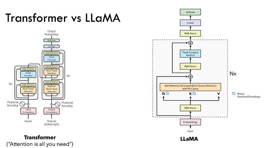
Figure1: Architecture Difference between Original Transformer and LLama (credit to Umar Jamil)
Examining Figure 1 reveals a profound shift from the original Transformer to the groundbreaking LLaMA architecture. LLaMA 2.0 is firmly rooted in the foundation of the Transformer framework, but it introduces distinct innovations — SwiGLU activation functions, rotary positional embeddings, root-mean-squared layer-normalization and key-value caching. In this blog, we will uncover the secrets behind LLaMA’s success and take you on a hands-on journey, coding the new architecture from scratch.
Quick Start
To dive right into action, our first step is installing the necessary library and importing the required packages. To get our hands dirty swiftly, I’ll begin by downloading a compact dataset from Hugging Face, providing us with a set of text sentences. These sentences will be transformed into tokens using the prebuilt tokenizer from ‘daryl149/llama-2–7b-chat-hf’ the very same tokenizer used during LLaMA’s pre-training.
!pip install transformers datasets SentencePieceimport random
import math
import numpy as np
import torch
import torch.nn as nn
from torch.nn import functional as F
from torch.utils.data import Dataset
from torch.utils.data.dataloader import DataLoader
from transformers import LlamaTokenizer
from datasets import load_dataset
This codebase serves as a concise example for running inference and highlighting the paradigm shift introduced by LLaMA 2.0 architecture. For a comprehensive implementation tailored for fine-tuning, I recommend exploring my previous article about Llama Fine Tuning with QLora. In this demonstration, we’ll grab a random batch of data from the dataset, there’s no need for constructing a pytorch DataLoader, as we won’t be training the model here.
model_id = "daryl149/llama-2-7b-chat-hf"
tokenizer = LlamaTokenizer.from_pretrained(model_id)
tokenizer.pad_token = tokenizer.eos_token

config = {
    ''vocab_size'': tokenizer.vocab_size,
    ''n_layers'': 1,
    ''embed_dim'': 2048,
    ''n_heads'': 32,
    ''n_kv_heads'': 8,
    ''multiple_of'': 64,
    ''ffn_dim_multiplier'': None,
    ''norm_eps'': 1e-5,
    ''max_batch_size'': 16,
    ''max_seq_len'': 64,
    ''device'': ''cuda'',
}

dataset = load_dataset(''glue'', ''ax'', split=''test'')
dataset = dataset.select_columns([''premise'', ''hypothesis''])

test_set = tokenizer(
    random.sample(dataset[''premise''], config[''max_batch_size'']),
    truncation=True,
    max_length=config[''max_seq_len''],
    padding=''max_length'',
    return_tensors=''pt''
)
Rotary Embedding
One of the fundamental advancements in LLaMA2 is the adoption of Rotary Position Embedding (RoPE) in place of traditional absolute positional encoding. What sets RoPE apart is its ability to seamlessly integrate explicit relative position dependencies into the self-attention mechanism of the model. This dynamic approach offers several key advantages:
- Flexibility in Sequence Length: Traditional position embeddings often require defining a maximum sequence length, limiting their adaptability. RoPE, on the other hand, is incredibly flexible. It can generate position embeddings on-the-fly for sequences of any length.
- Decaying Inter-Token Dependency: RoPE is smart about modeling the relationship between tokens. As tokens become more distant from each other in a sequence, RoPE naturally reduces their inter-token dependencies. This gradual decay aligns more closely with how humans understand language, where the importance of earlier words tends to diminish.
- Enhanced Self-Attention: RoPE equips the linear self-attention mechanisms with relative position encoding, a feature not present in traditional absolute positional encoding. This enhancement allows for more precise utilization of token embeddings.
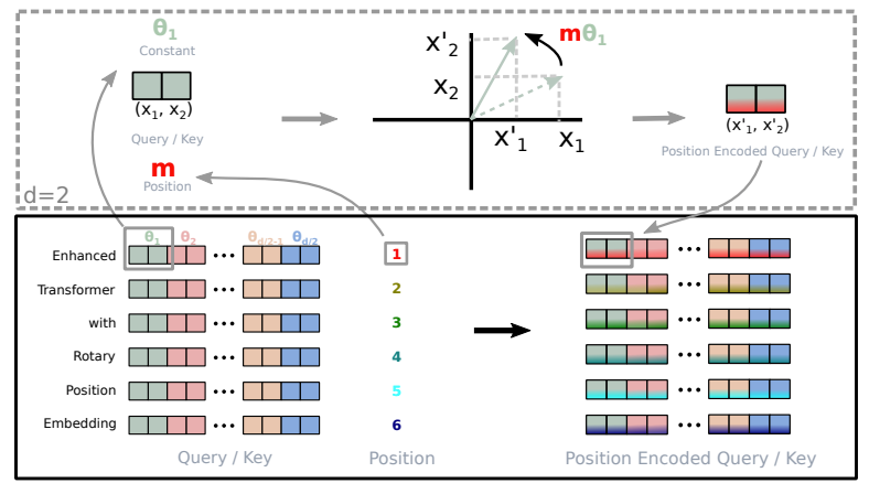
Implementation of Rotary Embedding (retrieved from Roformer)
Traditional absolute positional encoding would be akin to specifying that a word appears in position 3, 5, or 7, irrespective of the context. In contrast, RoPE lets the model understand how words are related to each other. It recognizes that word A often appears after word B and before word C. This dynamic understanding enhances the model’s performance.
def precompute_theta_pos_frequencies(head_dim, seq_len, device, theta=10000.0):

    # theta_i = 10000^(-2(i-1)/dim) for i = [1, 2, ... dim/2]
    # (head_dim / 2)
    theta_numerator = torch.arange(0, head_dim, 2).float()
    theta = 1.0 / (theta ** (theta_numerator / head_dim)).to(device)

    # (seq_len)
    m = torch.arange(seq_len, device=device)

    # (seq_len, head_dim / 2)
    freqs = torch.outer(m, theta).float()

    # complex numbers in polar, c = R * exp(m * theta), where R = 1:
    # (seq_len, head_dim/2)
    freqs_complex = torch.polar(torch.ones_like(freqs), freqs)
    return freqs_complex

def apply_rotary_embeddings(x, freqs_complex, device):

    # last dimension pairs of two values represent real and imaginary
    # two consecutive values will become a single complex number

    # (m, seq_len, num_heads, head_dim/2, 2)
    x = x.float().reshape(*x.shape[:-1], -1, 2)

    # (m, seq_len, num_heads, head_dim/2)
    x_complex = torch.view_as_complex(x)

    # (seq_len, head_dim/2) --> (1, seq_len, 1, head_dim/2)
    freqs_complex = freqs_complex.unsqueeze(0).unsqueeze(2)

    # multiply each complex number
    # (m, seq_len, n_heads, head_dim/2)
    x_rotated = x_complex * freqs_complex

    # convert back to the real number
    # (m, seq_len, n_heads, head_dim/2, 2)
    x_out = torch.view_as_real(x_rotated)

    # (m, seq_len, n_heads, head_dim)
    x_out = x_out.reshape(*x.shape)

    return x_out.type_as(x).to(device)
Let’s break down the code for Rotary Position Embedding (RoPE) to understand how it’s implemented.
precompute_theta_pos_frequenciesfunction calculates special values for RoPE. It starts by defining a hyperparameter calledthetathat controls the magnitude of the rotation. Smaller values create smaller rotations. Then, it computes a set of rotation angles usingtheta. The function also creates a list of positions within a sequence and calculates how much each position should rotate by taking the outer product of the position list and the rotation angles. Finally, it turns these values into complex numbers in polar form with a fixed magnitude, which is like a secret code for representing positions and rotations.apply_rotary_embeddingsfunction takes numerical values and augments them with rotation information. It starts by separating the last dimension of the input values into pairs representing the real and imaginary parts. These pairs are then combined into single complex numbers. Next, the function multiplies the precomputed complex numbers with the input, effectively applying a rotation. Finally, it converts the results back to real numbers and reshapes the data, making it ready for further processing.
RMSNorm
Llama2 adopts Root Mean Square Layer Normalization (RMSNorm), to enhance the transformer architecture by replacing the existing Layer Normalization (LayerNorm). LayerNorm has been beneficial for improving training stability and model convergence, as it re-centers and re-scales input and weight matrix values. However, this improvement comes at the cost of computational overhead, which slows down the network.

Simplified LayerNorm formula: Subtract the mean from the input and divide by the standard deviation
RMSNorm, on the other hand, retains the re-scaling invariance property while simplifying the computation. It regulates the combined inputs to a neuron using the root mean square (RMS), providing implicit learning rate adaptation. This makes RMSNorm computationally more efficient than LayerNorm.
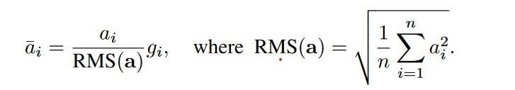 Formula for Root Mean Sqaure Normalization (RMSNorm) where gi is a gain parameter used to re-scale the standardized summed inputs
Extensive experiments across various tasks and network architectures show that RMSNorm performs as effectively as LayerNorm while reducing computation time by 7% to 64%.
class RMSNorm(nn.Module):
    def __init__(self, dim, eps=1e-6):
        super().__init__()
        self.eps = eps
        self.weight = nn.Parameter(torch.ones(dim))

    def _norm(self, x: torch.Tensor):
        # (m, seq_len, dim) * (m, seq_len, 1) = (m, seq_len, dim)
        # rsqrt: 1 / sqrt(x)
        return x * torch.rsqrt(x.pow(2).mean(-1, keepdim=True) + self.eps)

    def forward(self, x: torch.Tensor):
        # weight is a gain parameter used to re-scale the standardized summed inputs
        # (dim) * (m, seq_len, dim) = (m, seq_Len, dim)
        return self.weight * self._norm(x.float()).type_as(x)
This custom script first standardizes the input x, by dividing it by its root mean square, thereby making it invariant to scaling changes. The learned weight parameter self.weight is applied to each element in the standardized tensor. This operation adjusts the magnitude of the values based on the learned scaling factor.
KV Caching
Key-Value (KV) caching is a technique used to accelerate the inference process in machine learning models, particularly in autoregressive models like GPT and Llama. In these models, generating tokens one by one is a common practice, but it can be computationally expensive because it repeats certain calculations at each step. To address this, KV caching comes into play. It involves caching the previous Keys and Values, so we don’t need to recalculate them for each new token. This significantly reduces the size of matrices used in calculations, making matrix multiplications faster. The only trade-off is that KV caching requires more GPU memory (or CPU memory if a GPU isn’t used) to store these Key and Value states.
Attention with and without KV caching (Image created by João Lages)
Regarding the code, the KVCache class is responsible for handling this caching. It initializes two tensors, one for keys and one for values, both are initially filled with zeros. The update method is used to update the cache with new Key and Value information while the get method retrieves the cached Key and Value information based on the starting position and sequence length. This information can then be used for efficient attention calculations during token generation.
class KVCache:
    def __init__(self, max_batch_size, max_seq_len, n_kv_heads, head_dim, device):
        self.cache_k = torch.zeros((max_batch_size, max_seq_len, n_kv_heads, head_dim)).to(device)
        self.cache_v = torch.zeros((max_batch_size, max_seq_len, n_kv_heads, head_dim)).to(device)

    def update(self, batch_size, start_pos, xk, xv):
        self.cache_k[:batch_size, start_pos :start_pos + xk.size(1)] = xk
        self.cache_v[:batch_size, start_pos :start_pos + xv.size(1)] = xv

    def get(self, batch_size, start_pos, seq_len):
        keys = self.cache_k[:batch_size,  :start_pos + seq_len]
        values = self.cache_v[:batch_size, :start_pos + seq_len]
        return keys, values
During inference, the process operates on one token at a time, maintaining a sequence length of one. This means that, for Key, Value, and Query, both the linear layer and rotary embedding exclusively target a single token at a specific position. The attention weights are precomputed and stored for Key and Value as caches, ensuring that these calculations occur only once and their results are cached. The script getmethod retrieves past attention weights for Key and Value up to the current position, extending their length beyond 1. During the scaled dot-product operation, the output size matches the query size, which generate only a single token.
Grouped Query Attention
Llama incorporates a technique called grouped-query attention (GQA) to address memory bandwidth challenges during the autoregressive decoding of Transformer models. The primary issue stems from the need to load decoder weights and attention keys/values at each processing step, which consumes excessive memory.
In response, two strategies are introduced: and .
- Multi-query attention (MQA) involves utilizing multiple query heads with a single key/value head, which speeds up decoder inference. However, it has drawbacks such as quality degradation and training instability.
- Grouped-Query attention (GQA), is an evolution of MQA and strikes a balance by using an intermediate number of key-value heads (more than one but fewer than the query heads). The GQA model efficiently breaks the query into
n_headssegments like the original multi-head attention, and the key and value are divided inton_kv_headsgroups, enabling multiple key-value heads to share the same query.
By repeating key-value pairs for computational efficiency, the GQA approach optimizes performance while maintaining quality, as evidenced by the code implementation.
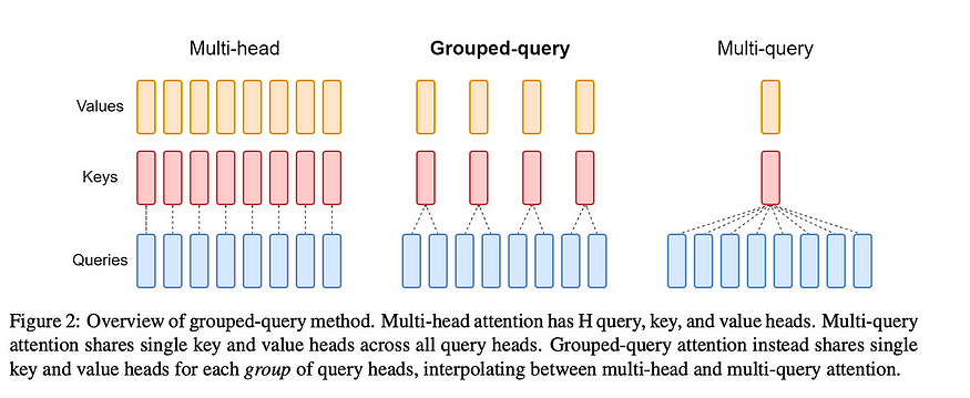
Overview of different Attention Method (introduced by Ainslie et al.)
The provided code is for implementing grouped query attention (GQA) within the context of an autoregressive decoder using a Transformer model. Notably, during inference, the sequence length (seq_len) is always set to 1.
def repeat_kv(x, n_rep):

    batch_size, seq_len, n_kv_heads, head_dim = x.shape
    if n_rep == 1:
        return x
    else:
        # (m, seq_len, n_kv_heads, 1, head_dim)
        # --> (m, seq_len, n_kv_heads, n_rep, head_dim)
        # --> (m, seq_len, n_kv_heads * n_rep, head_dim)
        return (
            x[:, :, :, None, :]
            .expand(batch_size, seq_len, n_kv_heads, n_rep, head_dim)
            .reshape(batch_size, seq_len, n_kv_heads * n_rep, head_dim)
        )

class SelfAttention(nn.Module):
    def __init__(self, config):
        super().__init__()

        self.n_heads = config[''n_heads'']
        self.n_kv_heads = config[''n_kv_heads'']
        self.dim = config[''embed_dim'']
        self.n_kv_heads = self.n_heads if self.n_kv_heads is None else self.n_kv_heads
        self.n_heads_q = self.n_heads
        self.n_rep = self.n_heads_q // self.n_kv_heads
        self.head_dim = self.dim // self.n_heads

        self.wq = nn.Linear(self.dim, self.n_heads * self.head_dim, bias=False)
        self.wk = nn.Linear(self.dim, self.n_kv_heads * self.head_dim, bias=False)
        self.wv = nn.Linear(self.dim, self.n_kv_heads * self.head_dim, bias=False)
        self.wo = nn.Linear(self.n_heads * self.head_dim, self.dim, bias=False)

        self.cache = KVCache(
            max_batch_size=config[''max_batch_size''],
            max_seq_len=config[''max_seq_len''],
            n_kv_heads=self.n_kv_heads,
            head_dim=self.head_dim,
            device=config[''device'']
        )

    def forward(self, x, start_pos, freqs_complex):

        # seq_len is always 1 during inference
        batch_size, seq_len, _ = x.shape

        # (m, seq_len, dim)
        xq = self.wq(x)

        # (m, seq_len, h_kv * head_dim)
        xk = self.wk(x)
        xv = self.wv(x)

        # (m, seq_len, n_heads, head_dim)
        xq = xq.view(batch_size, seq_len, self.n_heads_q, self.head_dim)

        # (m, seq_len, h_kv, head_dim)
        xk = xk.view(batch_size, seq_len, self.n_kv_heads, self.head_dim)
        xv = xv.view(batch_size, seq_len, self.n_kv_heads, self.head_dim)

        # (m, seq_len, num_head, head_dim)
        xq = apply_rotary_embeddings(xq, freqs_complex, device=x.device)

        # (m, seq_len, h_kv, head_dim)
        xk = apply_rotary_embeddings(xk, freqs_complex, device=x.device)

        # replace the entry in the cache
        self.cache.update(batch_size, start_pos, xk, xv)

        # (m, seq_len, h_kv, head_dim)
        keys, values = self.cache.get(batch_size, start_pos, seq_len)

        # (m, seq_len, h_kv, head_dim) --> (m, seq_len, n_heads, head_dim)
        keys = repeat_kv(keys, self.n_rep)
        values = repeat_kv(values, self.n_rep)

        # (m, n_heads, seq_len, head_dim)
        # seq_len is 1 for xq during inference
        xq = xq.transpose(1, 2)

        # (m, n_heads, seq_len, head_dim)
        keys = keys.transpose(1, 2)
        values = values.transpose(1, 2)

        # (m, n_heads, seq_len_q, head_dim) @ (m, n_heads, head_dim, seq_len) -> (m, n_heads, seq_len_q, seq_len)
        scores = torch.matmul(xq, keys.transpose(2, 3)) / math.sqrt(self.head_dim)

        # (m, n_heads, seq_len_q, seq_len)
        scores = F.softmax(scores.float(), dim=-1).type_as(xq)

        # (m, n_heads, seq_len_q, seq_len) @ (m, n_heads, seq_len, head_dim) -> (m, n_heads, seq_len_q, head_dim)
        output = torch.matmul(scores, values)

        # ((m, n_heads, seq_len_q, head_dim) -> (m, seq_len_q, dim)
        output = (output.transpose(1, 2).contiguous().view(batch_size, seq_len, -1))

        # (m, seq_len_q, dim)
        return self.wo(output)
SelfAttentionis a class that combines mechanism that we have discussed. The key components of this class are as follows:
- Linear transformations are applied to the input tensor for queries (xq), keys (xk), and values (xv). These transformations project the input data into a form suitable for processing.
- The rotary embedding is applied to the query, key, and value tensors using the provided frequency complex number. This step enhances the model’s ability to consider positional information and perform attention computations.
- The key-value pairs (k and v) are cached for efficient memory usage. The cached key-value pairs are retrieved up to current position (
start_pos + seq_len) - The query, key, and value tensors are prepared for Grouped-Query attention calculation by repeating key-value pairs
n_reptimes, wheren_repcorresponds to the number of query heads that share the same key-value pair. - Scaled dot-product attention computation. The attention scores are computed by taking the dot product of the query and key, followed by scaling. Softmax is applied to obtain the final attention scores. During the computation, the output size matches the query size, which is also 1.
- Finally, the module applies a linear transformation (
wo) to the output, and the processed output is returned.
SwiGlu
SwiGLU, as utilized in LLaMA2 models, is an activation function designed to enhance the performance of the position-wise feed-forward network (FFN) layers in the Transformer architecture. The main advantages of SwiGLU over other activation functions are:
- Smoothness: SwiGLU is smoother than ReLU, which can lead to better optimization and faster convergence.
- Non-monotonicity: SwiGLU is non-monotonic, which allows it to capture complex non-linear relationships between inputs and outputs
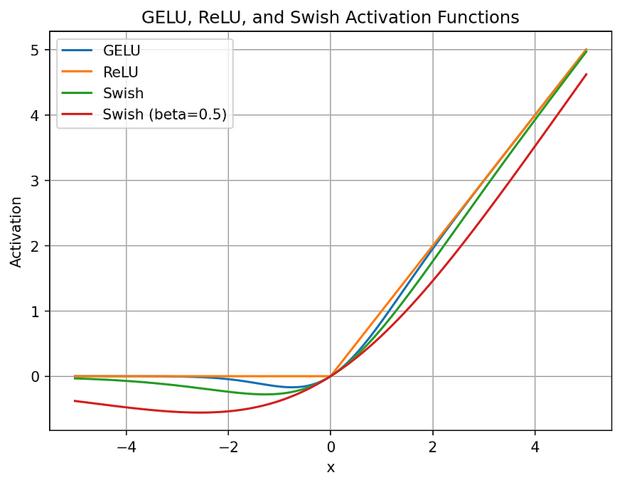
Comparison of different GLU activation (retrieved from KikaBeN)
def sigmoid(x, beta=1):
    return 1 / (1 + torch.exp(-x * beta))

def swiglu(x, beta=1):
    return x * sigmoid(x, beta)
Feedforward
In the Transformer architecture, the feedforward layer plays a crucial role, typically following the attention layer and normalization. The feedforward layer consists of three linear transformations.
class FeedForward(nn.Module):
    def __init__(self, config):

        super().__init__()

        hidden_dim = 4 * config[''embed_dim'']
        hidden_dim = int(2 * hidden_dim / 3)

        if config[''ffn_dim_multiplier''] is not None:
            hidden_dim = int(config[''ffn_dim_multiplier''] * hidden_dim)

        # Round the hidden_dim to the nearest multiple of the multiple_of parameter
        hidden_dim = config[''multiple_of''] * ((hidden_dim + config[''multiple_of''] - 1) // config[''multiple_of''])

        self.w1 = nn.Linear(config[''embed_dim''], hidden_dim, bias=False)
        self.w2 = nn.Linear(config[''embed_dim''], hidden_dim, bias=False)
        self.w3 = nn.Linear(hidden_dim, config[''embed_dim''], bias=False)

    def forward(self, x: torch.Tensor):
        # (m, seq_len, dim) --> (m, seq_len, hidden_dim)
        swish = swiglu(self.w1(x))
        # (m, seq_len, dim) --> (m, seq_len, hidden_dim)
        x_V = self.w2(x)

        # (m, seq_len, hidden_dim)
        x = swish * x_V

        # (m, seq_len, hidden_dim) --> (m, seq_len, dim)
        return self.w3(x)
During the forward pass, the input tensor x is subjected to multi layer of linear transformations. The SwiGLU activation function, applied after first transformation, enhances the expressive power of the model. The final transformation maps the tensor back to its original dimensions. This unique combination of SwiGLU activation and multiple FeedForward layer enhances the performance of the model.
Ultimate Transformer Model
The final culmination of Llama2, a powerful Transformer model, brings together the array of advanced techniques we’ve discussed so far. The DecoderBlock, a fundamental building block of this model, combines the knowledge of KV caching, Grouped Query Attention, SwiGLU activation, and Rotary Embedding to create a highly efficient and effective solution.
class DecoderBlock(nn.Module):
    def __init__(self, config):
        super().__init__()

        self.n_heads = config[''n_heads'']
        self.dim = config[''embed_dim'']
        self.head_dim = self.dim // self.n_heads

        self.attention = SelfAttention(config)
        self.feed_forward = FeedForward(config)

        # rms before attention block
        self.attention_norm = RMSNorm(self.dim, eps=config[''norm_eps''])

        # rms before  feed forward block
        self.ffn_norm = RMSNorm(self.dim, eps=config[''norm_eps''])

    def forward(self, x, start_pos, freqs_complex):

        # (m, seq_len, dim)
        h = x + self.attention.forward(
            self.attention_norm(x), start_pos, freqs_complex)
        # (m, seq_len, dim)
        out = h + self.feed_forward.forward(self.ffn_norm(h))
        return out

class Transformer(nn.Module):
    def __init__(self, config):
        super().__init__()
        self.vocab_size = config[''vocab_size'']
        self.n_layers = config[''n_layers'']
        self.tok_embeddings = nn.Embedding(self.vocab_size, config[''embed_dim''])
        self.head_dim = config[''embed_dim''] // config[''n_heads'']

        self.layers = nn.ModuleList()
        for layer_id in range(config[''n_layers'']):
            self.layers.append(DecoderBlock(config))

        self.norm = RMSNorm(config[''embed_dim''], eps=config[''norm_eps''])
        self.output = nn.Linear(config[''embed_dim''], self.vocab_size, bias=False)

        self.freqs_complex = precompute_theta_pos_frequencies(
            self.head_dim, config[''max_seq_len''] * 2, device=(config[''device'']))

    def forward(self, tokens, start_pos):
        # (m, seq_len)
        batch_size, seq_len = tokens.shape

        # (m, seq_len) -> (m, seq_len, embed_dim)
        h = self.tok_embeddings(tokens)

        # (seq_len, (embed_dim/n_heads)/2]
        freqs_complex = self.freqs_complex[start_pos:start_pos + seq_len]

        # Consecutively apply all the encoder layers
        # (m, seq_len, dim)
        for layer in self.layers:
            h = layer(h, start_pos, freqs_complex)
        h = self.norm(h)

        # (m, seq_len, vocab_size)
        output = self.output(h).float()
        return output

model = Transformer(config).to(config[''device''])
res = model.forward(test_set[''input_ids''].to(config[''device'']), 0)
print(res.size())
The Transformer model encompasses a stack of DecoderBlocks to create a robust and efficient deep learning architecture. The accompanying code showcases how the DecoderBlock, with its SelfAttention, FeedForward, and RMSNorm layers, effectively processes data. The code also highlights the larger Transformer architecture’s structure, including token embeddings, layer stacking, and output generation. Furthermore, the use of precomputed frequencies and advanced techniques, combined with customized configurations, ensures the model’s remarkable performance and versatility in various natural language understanding tasks.
Conclusion
In this comprehensive journey through Llama2’s advanced techniques for Transformers, we’ve delved into both the theory and the intricate code implementation. However, it’s important to note that the code we’ve discussed is not primarily for training or production use but serves more as a demonstration and showcase of Llama’s remarkable inference ability. It highlights how these advanced techniques can be applied in a real-world context and showcases the potential of Llama2 in enhancing various natural language understanding tasks.
Thank You
🌟 If you found this article meaningful and would like to stay updated on my future articles, please consider following me on Medium. I’m excited to share more valuable insights and engaging content with you in the coming weeks.
Comments
Loading comments…