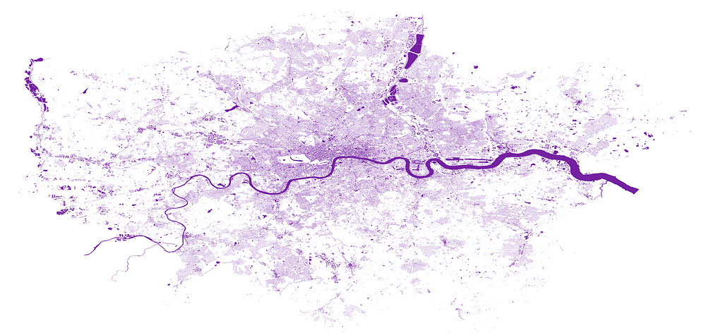
Tha above image resembles buildings in London (data source OpenStreetMap), displayed using GeoPandas and Matplotlib.
Geopandas is a powerful tool when it comes to analysing geospatial data using Python. Based on Pandas, GeoPandas offers us not only the ability to filter, sort and manipulate data, but also perform spatial queries, manipulations, and importantly, built in plotting. This makes data validation and exploration quick and simple.
In this article I will show a quick and easy way to load a downloaded OSM data file into a GeoDataFrame ready for exploring and analysing.
Installing dependencies
Other than Python and GeoPandas, the main requirement will be ogr2ogr, a CLI tool included in GDAL.
Downloading GDAL is made simple using the package manager conda, which is easily installed using Miniconda — conda’s lightweight installer. The benefit of this approach is it is platform neutral (should work on Mac, Windows, Linux — if you are using Linux however, you can also try using your main package manager to install gdal-bin).
As always, it is a good idea to create a new environment for your project to avoid dependency clashes. Once conda is set up, installing gdal (and GeoPandas) should be as simple as running:
conda install -c conda-forge gdal geopandas
Note: -c conda-forge specifies installing from the conda-forge channel. This is the channel where GDAL is available.
We will also be using the Python libraries requests, Pandas (included in GeoPandas), and Jupyter lab.
Once our set up is ready, start Jupyter lab/notebook and try importing the required packages. You can also confirm that GDAL successfully installed by checking the version of ogr2ogr.
I am using Google Colab for the purposes of this article, so the first two lines shown here are installation. These will vary for your local set up (requests, for example, is included in the Google Colab environment by default and therefore doesn’t need installing).
Confirming required dependencies are installed:
!pip3 install geopandas
!apt-get install gdal-bin

import requests
import sqlite3
import geopandas as gpd
import pandas as pd

!ogr2ogr --version
GDAL 3.3.2, released 2021/09/01
Note sqlite3 is included in the Python standard library so doesn’t need installing.
Once dependencies are installed and working, we are ready to download our data. I will be downloading .osm.pbf data for London from Geofabrik, my preferred source of OpenStreetMap data. I choose to use the CLI tool wget for downloading by running the following line from within my notebook:
!wget http://download.geofabrik.de/europe/great-britain/england/greater-london-latest.osm.pbf -O london-latest.osm.pbf
You should see a progress bar as the output. When this reaches 100%, we are ready to move on to the next step; converting the .osm.pbf into a more easily accessible format.
Import data into sqlite database file using ogr2ogr
Now that we have an .osm.pbf file containing our area of interest, we are ready to convert the file into a more easily accessible format. Python comes with a built in module for reading SQLite files, which makes using sqlite a great choice.
The following command in your notebook will load the downloaded .osm.pbf file into a SQLite database file.
!ogr2ogr -f SQLite -lco FORMAT=WKT london.sqlite london-latest.osm.pbf
ogr2ogr supports a large number of geospatial vector file formats. I have chosen SQLite because:
- It requires no further set up (no pre-existing database required)
- As mentioned, SQLite files are easily readable using Python thanks to the sqlite3 module
- Pandas supports loading data from SQL sources
- It is memory efficient and suitable for larger datasets (unlike e.g. GeoJson)
Note the -lco parameter here controls the format of geometry column within the outputted london.sqlite file. I have chosen WKT (Well Known Text format).
Once the progress bar reaches 100, we are ready to continue. Since we don’t know the schema for the data, we will do some exploring first to discover the table names.
Following on from the first block, see the next few steps and query to view table names below. (sqlite_master contains the schema; we are querying for all tables related to our geometry data).
Downloading data, converting to sqlite and viewing table names:
Check the GitHub gist here: connect-sqlite.ipynb
Note the outputted table names:
[('geometry_columns',),
 ('spatial_ref_sys',),
 ('points',),
 ('lines',),
 ('multilinestrings',),
 ('multipolygons',),
 ('other_relations',)]
Thanks to Panda’s read_sql method, loading our data into a Pandas DataFrame makes checking the contents of the tables much easier. This means we won’t have to directly parse results of sqlite3’s cursor ourselves.
Taking a look at the ‘geometry_columns’ and ‘spatial_ref_sys’ tables, we can see the following:
Exploring data in geometry_columns, spatial_ref_sys tables and previewing points table: explore-tables.ipynb
The geometry_column table contains useful metadata about our geometries and is created by SQLite, or to be specific, Spatialite — SQLite’s geoextension. The column geometry_type here references the type of geometry, and should match the table name.
For reference, Spatialite geometry_types have the following values (taken from https://www.gaia-gis.it/gaia-sins/BLOB-Geometry.html)
1 = POINT
2 = LINESTRING
3 = POLYGON
4 = MULTIPOINT
5 = MULTILINESTRING
6 = MULTIPOLYGON
7 = GEOMETRYCOLLECTION
Something to note about our data is that we are missing polygons and multipoints. It turns out there are multipolygons in the multipolygon table that actually only contain one polygon. This seems to be how the OSM elements are matched to Spatialite types.
Lastly, the spatial_ref_sys shows us which Spatial Reference System is being used; in our case 4326, a standard in web maps.
Loading the data into a GeoDataFrame
We are now ready to start exploring the interesting part of our data — the geometries. To do this, we will first load our data into a GeoDataFrame for easier plotting and spatial querying.
We have already seen how to load the data into a Panda’s DataFrame. To geo-enable our dataframe we need to convert the geometry column from a string (currently a WKT string) to a geometry object. In the case of GeoPandas, our geometry object will be a Shapely object under the hood.
For simplicity, I have gathered all geometry types into one dataframe and included a table_name column for reference. We need to import Shapely’s wkt module in order for the from_wkt method to work (Shapely can read the geometry from our WKT string).
Creating a GeoDataFrame from our Panads DataFrame:
Check out the GitHub gist here: geodataframe.ipynb
Notice in the second block that we are first creating a GeoSeries (geometry column) in our DataFrame using the GeoSeries.from_wkt() method, and then creating a GeoDataFrame using this. In the GeoDataFrame output, we can see this added column, named ‘geom’, with the dtype geometry.
We can now turn our attention to the contents of our GeoDataFrame.
Exploring our OSM data using GeoPandas
OSM data is organised using tags. We can check the Wiki for details on tag usage and what they mean. I will be using some basic examples to illustrate.
Before we start looking into the tags, let’s first of all see what our data looks like. London is not only largely populated — almost 9 million inhabitants — it also covers a large area of 1,572.03 km2. This makes it both the largest population and area in of cities in western Europe (excluding Moscow and Istanbul). In OSM terms, Greater London has a total of 88MB, which is reasonable but not huge. It is large enough however to create a mess when trying to view everything at once. The result of the following command can be seen below. (The column parameter sets the column used for colouring.)
# Plotting all our data
gdf.plot(figsize=(25,25), column='ogc_fid')
Entire OSM data for Greater London plotted using GeoPandas:
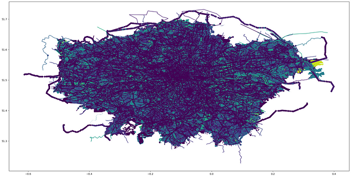
As you can see, the result is not very legible. It does show us, however, that the previous steps worked; our geometries are there and the shape looks like London, albeit a bit squashed. The squashing is a byproduct of the Spatial Reference System mentioned earlier (a common issue). Filtering some of the layers will help make our data easier to interpret.
# viewing landuse
condition = gdf['landuse'].notnull()
gdf[condition].plot(figsize=(50,50), column="landuse", legend=True)
Landuse in London with legend:
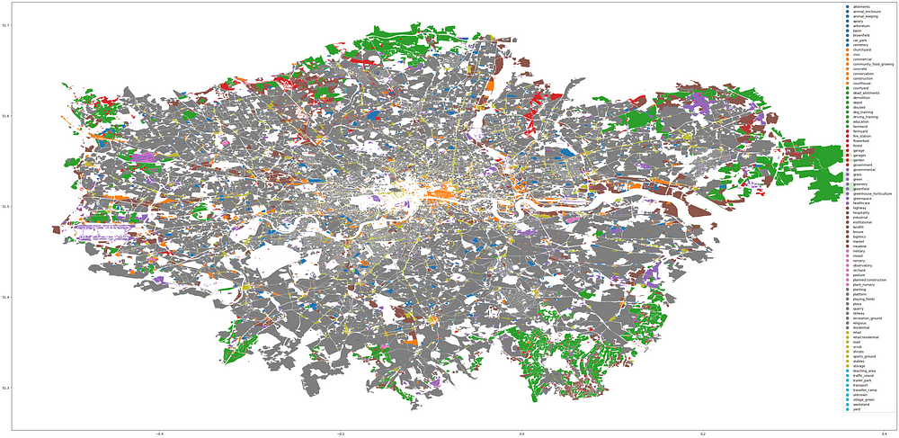
By filtering based on the presence of data in one of the columns (in this case the ‘landuse’ column), we can limit the results to only show geometries tagged with that particular key. We aren’t yet filtering by value; notnull() will only check whether there is a value or not. In this case all landuse geometries will be shown.
Due to the large number of values, the legend is small — but we can see that grey dominates the map here, meaning that — among others — retail and residential are the most common landuse types.
Answering a question with our data: which London borough has the highest density of green space?
We have done some basic checking of our data. Now we can start answering some questions. As an example, I will be answering the question: which London borough has the highest density of green space? For my purposes (and to make things simple) ‘green space’ will be a park or nature reserve.
Let’s firstly see what that looks like:
# values for 'leisure' include 'park' and 'nature_reserve'
condition = gdf['leisure'].isin(['park', 'nature_reserve'])
gdf[condition].plot(figsize=(50,50), color="green")
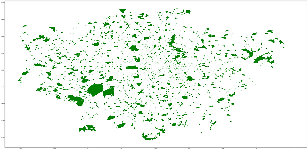
London parks and nature reserves:
Tip: to see the all the available values for a tag (within the data), try using the Pandas.Series.unique() method.
It looks like there is a broad distribution of parks, with Richmond Park dominating the south west. There are lots of smaller parks that we lose sight of when looking at an overview like this. We need some numbers to confirm our suspicion — that the borough containing Richmond Park (London Borough of Richmond) has have the highest density of green space.
This is where GeoPandas is a huge convenience. Not only can we easily measure the area of all our green space geometries using the .area attribute -since the geometry column contains Shapely geometries, we don’t need to do the calculating ourselves- but we can also use the London borough outlines to clip the parks to the relevant areas.
Rough outline of the steps:
- Filter to borough geometries
- Clip parks to boroughs
- Calculate area of parks in each borough
- Calculate area of each borough
- Create DataFrame of park/borough area density
Filtering green space geometries and borough polygons:
Check out the GitHub gist here: boroughs.ipynb
We now have GeoDataFrames containing green space geometries and London borough polygons. Checking the names of the administrative boundaries ensures we are selecting the right ones; without using using admin_level for filtering, the polygon for entire Greater London was included, as well as some smaller sub-borough divisions. By manually checking the data we can decide on the best tag for filtering.
Now we have the information we need to calculate the percentage of total area covered by green space for each borough. Since there are not many boroughs, this can be acheived by looping through each one and making use of GeoPanda’s built in GeoPandas.clip() function and GeoSeries.area attribute.
Calculating green space density for each London borough:
Check out the GitHub gist: green-spaces-boroughs.ipynb
As suspected, Richmond comes in top at approximately 36%, thanks for the most part to Richmond Park. Second is Merton, followed by Westminster and Hackney. City of London — the innermost borough and techincally not a borough at all — comes last.
I have focused on parks and nature reserves for the purpose of this task. It could be that other green spaces are being missed by over simplifying the critieria. More exploration is needed to determine this. Another interesting follow up task could be to supplement this data with information about resident demographics and property prices prices within each borough. Aside from geographic factors - boroughs further out of the city center are likely to be ‘greener’ - there may well be other correlations to discover.
Comments
Loading comments…