Introduction
Numerical integration is the process of using numerical techniques to solve an integral. This article demonstrates how to evaluate a function’s integral numerically using Python.
The fundamental theorem of calculus proves the link between derivatives, integration, and the area under curves. Review Numerical Differentiation in Python if necessary before proceeding.
Theory
Integrating a function over a specific interval [a, b] effectively finds the area under the curve between a and b.
The definite integral is given by Equation 1:

Similar to differentiation, many techniques can be applied to find the analytical solution for a definite antiderivative. However, sometimes there are obstacles in the way of using these techniques. For example, it is impossible to express the antiderivative of some functions in terms of known functions in some cases.
Techniques
Obtaining or approximating a region enclosed between the x-axis and a curve f(x) is equivalent to a Riemann sum by adding up numerous portions of smaller areas comprising this more extensive area.
Presented below are Python implementations of three of the most common numerical integration techniques:
- Trapezoidal Rule
- Midpoint Rule
- Simpson’s Rule
Each numerical integration technique mentioned requires the calculation of the continuous function f(x) at a set of n+1 equally spaced points on the interval [a, b].
Equation 2 shows how to calculate the step between each point:

The most computationally efficient numerical integration techniques reach a sufficient integral value approximation using the least amount of f(x) evaluations.
Trapezoidal Rule
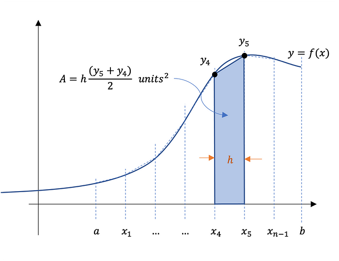
A trapezoid is a four-sided polygon with a pair of parallel sides, whose area is given by Equation 3:

Figure 1 illustrates the area segmentation using n trapezoids. Summing the individual areas of each trapezoid approximates the total area.
Figure 1 — Trapezoidal Rule:
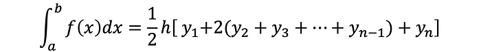
Equation 4 is the numerical integration trapezoidal rule and Gist 1 shows its Python implementation with comments summarizing each step.
Gist 1 — Trapezoidal Rule Python Code
# ==============================================================
# trapezoidal rule

def trapezoid(a, b, n):
	"""
	trapezoidal rule numerical integral implementation
	a: interval start
	b: interval end
	n: number of steps
	return: numerical integral evaluation
	"""

	# initialize result variable
	res = 0

	# calculate number of steps
	h = (b - a) / n

	# start at a
	x = a

	# sum 2*yi (1 ≤ i ≤ n-1)
	for _ in range(1, n):
	x += h
	res += f(x)
	res *= 2

	# evaluate function at a and b and add to final result
	res += f(a)
	res += f(b)

	# divide h by 2 and multiply by bracketed term
	return (h / 2) * res
Midpoint Rule
The midpoint rule for estimating a definite integral uses a Riemann sum of rectangles with subintervals of equal width. The height of each rectangle corresponds to f(x) evaluated at the midpoints of the n subintervals.
Figure 2 depicts the subintervals, the midpoints, and the rectangles:

Equation 5 calculates the midpoints:
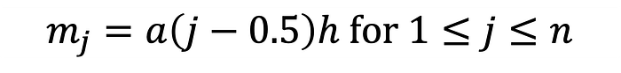
Recall that a is the start of the interval, and h is the step size. n is the number subintervals. Equation 6 gives the midpoint rule:
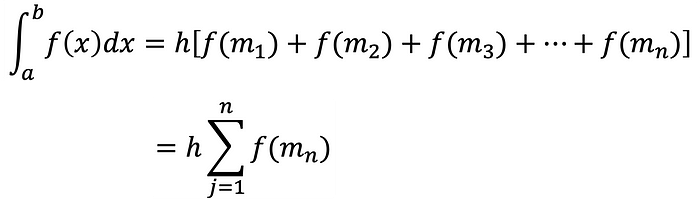
Summing the areas of rectangles approximates the area between the graph of f(x) and the x-axis over the specified interval.
Gist 2 shows the Python code for the midpoint rule:
# ==============================================================
# midpoint rule

def midpoint(a, b, n):
	"""
	midpoint rule numerical integral implementation
	a: interval start
	b: interval end
	n: number of steps
	return: numerical integral evaluation
	"""

	# initialize result variable
	res = 0

	# calculate number of steps
	h = (b - a) / n

	# starting midpoint
	x = a + (h / 2)

	# evaluate f(x) at subsequent midpoints
	for _ in range(n):
		res += f(x)
		x += h

	# multiply final result by step size
	return h * res
The Trapezoidal Rule and Midpoint Rule are Riemann summation techniques that use linear functions to approximate the integral.
Simpson’s Rule
Simpson’s rule approximates the value of a definite integral by using quadratic functions. Therefore, better integral approximations are expected compared to the previous techniques covered.
Equation 7 is Simpson’s rule for numerical integration:
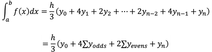
Needed is a minimum of three sampling points to use Simpson’s rule. So the total number of sampling points, in general, must be odd, i.e. the number n of subintervals must be even.
Gist 3 shows the Python code for Simpson’s rule:
# ==============================================================
# simpson's rule

def simpsons(a, b, n):
	"""
	simpson's rule numerical integral implementation
	a: interval start
	b: interval end
	n: number of steps
	return: numerical integral evaluation
	"""

	# calculate number of steps
	h = (b - a) / n

	# start at a
	x = a

	# store f(x) evaluation at start and end
	res = f(x)
	res += f(b)

	# sum [2*yi (i is even), 4*yi (i is odd)]
	for i in range(1, n):
		x += h
		res += 2 * f(x) if i % 2 == 0 else 4 * f(x)

	# divide h by 3 and multiply for final result
	return (h / 3) * res
Error Estimations
Two important metrics to assess the performance of the techniques are the approximation error and _computation tim_e.
Let f(x) be the function given in Equation 8:

Equation 9 is the analytical integral used in this analysis for demonstration purposes. As mentioned, numerical integration is usually employed when an analytical solution does not exist.

The interval for the analysis is chosen arbitrarily to be [2, 10], and the expected value to 17 significant figures is 1.6094379124341005.
The estimation error is an expression of the difference between the measured value and the expected value, determined using Equation 10:

In this case, the measured value is the numerical integration approximation.
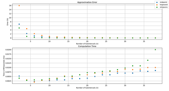
Figure 3 shows a plot of the errors and computation time for the trapezoidal, midpoint, and Simpson’s rule applied to Equation 8 to approximate Equation 9 for increasing numbers of subintervals.
Conclusion
Results show that as the number of subintervals increases, computation time increases, and error reduces. Note that the Python implementations do not focus on performance optimization, so improvements are likely possible.
Simpson’s rule appears to produce the most accurate approximations however is the most computationally expensive.
This article has demonstrated numerical integration in Python using the trapezoidal, midpoint, and Simpson’s rules.
Thank you for reading.
Comments
Loading comments…