Working with PDB files in Python

Unlock the secrets of protein structures with Python! This article will guide you through the fascinating world of molecular biology, focusing on the manipulation and visualization of Protein Data Bank (PDB) files --- an essential resource for applications like drug design and protein engineering. If you're comfortable with Python and Pandas, you're already halfway there!

The main point of this tutorial is to show how we can manipulate PDB data with the usual PyData Stack, especially Pandas dataframes (so you don't need to learn an entirely new API) and how we can simply visualize the proteins.

What is a PDB file?

A PDB (Protein Data Bank) file is a standardized text-based file format that stores the three-dimensional (3D) structural data of biological macromolecules, primarily proteins and nucleic acids, as well as their complexes. These files contain the atomic coordinates, bond information, and other relevant details of the biomolecules derived from experimental methods...

The common PDB keys are:

1. HEADER: Provides a general description of the contents of the PDB file, including the name of the macromolecule, classification, deposition date, and PDB ID.
2. TITLE: Gives a more detailed description of the structure, often including the protein's function, any ligands or cofactors, and relevant experimental conditions.
3. COMPND: Describes the macromolecular components of the structure, such as the names of individual protein chains, nucleic acids, or ligands.
4. SOURCE: Specifies the natural or synthetic source of each macromolecular component, including the organism, tissue, or cell line from which the structure was derived.
5. KEYWDS: Lists keywords that describe the structure, such as enzyme classification, protein family, or biological process.
6. EXPDTA: Provides information about the experimental method used to determine the structure, such as X-ray crystallography, NMR spectroscopy, or cryo-electron microscopy.
7. AUTHOR: Lists the names of the researchers who contributed to the structure determination and submitted the PDB file.
8. REVDAT: Records the revision history of the PDB file, including the dates of modifications and a brief description of the changes made.
9. JRNL: Contains citation information for the publication(s) associated with the structure determination, such as the title, authors, journal name, volume, pages, and publication year.
10. REMARK: Contains various remarks or comments related to the structure, such as experimental details, data processing, model quality, and other relevant notes.
11. SEQRES: Describes the primary sequence of each protein or nucleic acid chain in the structure, listing the amino acid or nucleotide residues in one-letter codes.
12. CRYST: Unit cell parameters, space group, and Z value. If the structure was not determined by crystallographic means, simply defines a unit cube
13. ORIGXn: (n=1, 2, 3) Defines the transformation from the orthogonal coordinates contained in the database entry to the submitted coordinates
14. SCALEn: (n=1,2, 3) Defines the transformation from the orthogonal coordinates contained in the entry to fractional crystallographic coordinates.
15. ATOM: Contains the atomic coordinates for each non-hydrogen atom in the macromolecule, including information such as the atom name, residue name, chain identifier, residue number, and occupancy.
16. HETATM: Similar to the ATOM record, but for non-standard residues, such as ligands, cofactors, or modified amino acids.
17. HELIX and SHEET: Provide information about the secondary structure elements, such as alpha-helices and beta-sheets, specifying the residues involved and their chain identifiers.
18. TER: Indicates the end of a protein or nucleic acid chain in the coordinate records, allowing for the separation of different chains in the structure.
19. CONECT: Lists the connectivity information for covalent and non-covalent bonds in the structure, including disulfide bridges, metal coordination sites, and bonds between standard and non-standard residues.
20. MASTER: Provides a summary of the number of lines for various record types in the PDB file, often found just before the END record.

An example of part of the 3NIR protein file (atoms 26 to 1026 are removed):

HEADER PLANT PROTEIN 16-JUHEADER PLANT PROTEIN 16-JUN-10 3NIR
TITLE CRYSTAL STRUCTURE OF SMALL PROTEIN CRAMBIN AT 0.48 A RESOLUTION
COMPND MOL_ID: 1;
COMPND 2 MOLECULE: CRAMBIN;
COMPND 3 CHAIN: A
SOURCE MOL_ID: 1;
SOURCE 2 ORGANISM_SCIENTIFIC: CRAMBE HISPANICA;
SOURCE 3 ORGANISM_COMMON: ABYSSINIAN CRAMBE, ABYSSINIAN KALE;
SOURCE 4 ORGANISM_TAXID: 3721;
SOURCE 5 STRAIN: SUBSP. ABYSSINICA
KEYWDS PLANT PROTEIN
EXPDTA X-RAY DIFFRACTION
AUTHOR A.SCHMIDT,M.TEETER,E.WECKERT,V.S.LAMZIN
REVDAT 5 04-APR-18 3NIR 1 REMARK
REVDAT 4 24-JAN-18 3NIR 1 JRNL
REVDAT 3 08-NOV-17 3NIR 1 REMARK
REVDAT 2 02-MAR-16 3NIR 1 SEQADV SEQRES VERSN
REVDAT 1 18-MAY-11 3NIR 0
JRNL AUTH A.SCHMIDT,M.TEETER,E.WECKERT,V.S.LAMZIN
JRNL TITL CRYSTAL STRUCTURE OF SMALL PROTEIN CRAMBIN AT 0.48 A
JRNL TITL 2 RESOLUTION
JRNL REF ACTA CRYSTALLOGR.,SECT.F V. 67 424 2011
JRNL REFN ESSN 1744-3091
JRNL PMID 21505232
JRNL DOI 10.1107/S1744309110052607
REMARK 1
REMARK 1 REFERENCE 1
REMARK 1 AUTH C.JELSCH,M.M.TEETER,V.S.LAMZIN,V.PICHON-PESME,R.H.BLESSING,
REMARK 1 AUTH 2 C.LECOMTE
REMARK 1 TITL ACCURATE PROTEIN CRYSTALLOGRAPHY AT ULTRA-HIGH RESOLUTION:
REMARK 1 TITL 2 VALENCE ELECTRON DISTRIBUTION IN CRAMBIN.
REMARK 1 REF PROC.NATL.ACAD.SCI.USA V. 97 3171 2000
REMARK 1 REFN ISSN 0027-8424
REMARK 1 PMID 10737790
REMARK 2
REMARK 2 RESOLUTION. 0.48 ANGSTROMS.
REMARK 3
REMARK 3 REFINEMENT.
REMARK 3 PROGRAM : MOPRO
REMARK 3 AUTHORS : GUILLOT,VIRY,GUILLOT,LECOMTE,JELSCH
DBREF 3NIR A 1 46 UNP P01542 CRAM_CRAAB 1 46
SEQADV 3NIR SER A 22 UNP P01542 PRO 22 MICROHETEROGENEITY
SEQADV 3NIR ILE A 25 UNP P01542 LEU 25 MICROHETEROGENEITY
SEQRES 1 A 46 THR THR CYS CYS PRO SER ILE VAL ALA ARG SER ASN PHE
SEQRES 2 A 46 ASN VAL CYS ARG LEU PRO GLY THR PRO GLU ALA LEU CYS
SEQRES 3 A 46 ALA THR TYR THR GLY CYS ILE ILE ILE PRO GLY ALA THR
SEQRES 4 A 46 CYS PRO GLY ASP TYR ALA ASN
HET EOH A2001 3
HET EOH A2002 6
HET EOH A2003 6
HET EOH A2004 3
HETNAM EOH ETHANOL
FORMUL 2 EOH 4(C2 H6 O)
FORMUL 6 HOH \*98(H2 O)
HELIX 1 1 SER A 6 LEU A 18 1 13
SHEET 1 A 2 THR A 2 CYS A 3 0
SHEET 2 A 2 ILE A 33 ILE A 34 -1 O ILE A 33 N CYS A 3
SSBOND 1 CYS A 3 CYS A 40 1555 1555 2.03
SSBOND 2 CYS A 4 CYS A 32 1555 1555 2.05
SSBOND 3 CYS A 16 CYS A 26 1555 1555 2.04
SITE 1 AC1 8 ALA A 45 ASN A 46 EOH A2004 HOH A3006
SITE 2 AC1 8 HOH A3027 HOH A3038 HOH A3087 HOH A3091
SITE 1 AC2 10 ILE A 7 VAL A 8 SER A 11 ALA A 27
SITE 2 AC2 10 GLY A 31 CYS A 32 ILE A 33 HOH A3002
SITE 3 AC2 10 HOH A3068 HOH A3102
SITE 1 AC3 3 ILE A 7 ASN A 46 HOH A3063
SITE 1 AC4 7 ASN A 14 LEU A 18 EOH A2001 HOH A3011
SITE 2 AC4 7 HOH A3020 HOH A3023 HOH A3085
CRYST1 22.329 18.471 40.769 90.00 90.55 90.00 P 1 21 1 2
ORIGX1 1.000000 0.000000 0.000000 0.00000
ORIGX2 0.000000 1.000000 0.000000 0.00000
ORIGX3 0.000000 0.000000 1.000000 0.00000
SCALE1 0.044785 0.000000 0.000430 0.00000
SCALE2 0.000000 0.054139 0.000000 0.00000
SCALE3 0.000000 0.000000 0.024530 0.00000
ATOM 1 N ATHR A 1 3.265 -14.107 16.877 0.87 4.71 N
ATOM 2 N BTHR A 1 4.046 -14.111 17.614 0.25 9.35 N
ATOM 3 CA ATHR A 1 4.047 -12.839 16.901 0.76 3.80 C
ATOM 4 CA BTHR A 1 4.261 -12.797 17.017 0.20 4.94 C
ATOM 5 C ATHR A 1 4.817 -12.834 15.587 0.80 3.68 C
ATOM 6 C BTHR A 1 4.935 -12.642 15.657 0.22 3.77 C
ATOM 7 O ATHR A 1 5.379 -13.834 15.145 0.85 5.76 O
ATOM 8 O BTHR A 1 5.025 -13.745 15.106 0.16 5.61 O
ATOM 9 CB ATHR A 1 5.042 -12.868 18.075 0.65 4.22 C
ATOM 10 CB BTHR A 1 4.850 -11.840 18.069 0.25 9.70 C
ATOM 11 OG1ATHR A 1 4.228 -13.043 19.244 0.78 6.21 O
ATOM 12 OG1BTHR A 1 4.711 -10.458 17.718 0.25 10.60 O
ATOM 13 CG2ATHR A 1 5.890 -11.610 18.173 0.63 5.67 C
ATOM 14 CG2BTHR A 1 6.341 -12.129 18.134 0.25 9.55 C
ATOM 15 H1 ATHR A 1 3.035 -14.005 16.173 0.75 6.58 H
ATOM 16 H1 BTHR A 1 2.914 -14.713 18.488 0.25 11.77 H
ATOM 17 H2 ATHR A 1 2.830 -14.148 17.523 0.75 6.58 H
ATOM 18 H2 BTHR A 1 4.980 -14.983 15.512 0.25 11.77 H
ATOM 19 H3 ATHR A 1 3.680 -15.162 17.238 0.75 6.58 H
ATOM 20 H3 BTHR A 1 9.013 -8.192 18.474 0.25 11.77 H
ATOM 21 HA ATHR A 1 3.181 -11.806 16.823 0.75 4.19 H
ATOM 22 HA BTHR A 1 3.605 -12.290 17.060 0.25 5.98 H
ATOM 23 HB ATHR A 1 5.699 -13.731 17.989 0.75 4.53 H
ATOM 24 HB BTHR A 1 4.523 -12.115 19.103 0.25 9.37 H
ATOM 25 HG1ATHR A 1 3.314 -12.887 19.057 0.75 8.30 H
HETATM 1027 O HOH A3123 21.546 -12.379 16.777 1.00 61.40 O
CONECT 66 795
CONECT 76 633
CONECT 324 515
CONECT 515 324
CONECT 633 76
CONECT 795 66
CONECT 894 895 896
CONECT 895 894
CONECT 896 894
CONECT 897 899 901
CONECT 898 900 902
CONECT 899 897
CONECT 900 898
CONECT 901 897
CONECT 902 898
CONECT 903 905 907
CONECT 904 906 908
CONECT 905 903
CONECT 906 904
CONECT 907 903
CONECT 908 904
CONECT 909 910 911
CONECT 910 909
CONECT 911 909
MASTER 322 0 4 1 2 0 8 6 451 1 24 4
END

Loading in PDB files

For this part, we're going to use BioPandas and ProDy, you can install them in your python environment using pip:

pip install biopandas prody

Here is a handy all-in-one function that reads a PDB file from a file path or a PDB/Uniprot ID into a pandas DataFrame, this is adapted from the Graphein package:

import pandas as pd
from biopandas.pdb import PandasPdb
from prody import parsePDBHeader
from typing import Optional

def read_pdb_to_dataframe(
pdb_path: Optional[str] = None,
model_index: int = 1,
parse_header: bool = True, ) -> pd.DataFrame:
"""
Read a PDB file, and return a Pandas DataFrame containing the atomic coordinates and metadata.

    Args:
        pdb_path (str, optional): Path to a local PDB file to read. Defaults to None.
        model_index (int, optional): Index of the model to extract from the PDB file, in case
            it contains multiple models. Defaults to 1.
        parse_header (bool, optional): Whether to parse the PDB header and extract metadata.
            Defaults to True.

    Returns:
        pd.DataFrame: A DataFrame containing the atomic coordinates and metadata, with one row
            per atom
    """
    atomic_df = PandasPdb().read_pdb(pdb_path)
    if parse_header:
        header = parsePDBHeader(pdb_path)
    else:
        header = None
    atomic_df = atomic_df.get_model(model_index)
    if len(atomic_df.df["ATOM"]) == 0:
        raise ValueError(f"No model found for index: {model_index}")

    return pd.concat([atomic_df.df["ATOM"], atomic_df.df["HETATM"]]), header

This function integrates the ability to parse the PDB header in the form of a dictionary that allows it to store all the useful information that needs to be used in downstream tasks.

Using our previous example (download 3nir.pbd):

df, df_header = read_pdb_to_dataframe('3nir.pdb')
df.head(10)

> > > print(df.shape)
> > > (1026, 22)
> > > print(df_header.keys())
> > > dict_keys(['helix', 'helix_range', 'sheet', 'sheet_range', 'chemicals', 'polymers', 'reference', 'resolution', 'biomoltrans', 'version', 'deposition_date', 'classification', 'identifier', 'title', 'experiment', 'authors', 'space_group', 'related_entries', 'EOH', 'A'])

Now dfis a just vanilla Pandas dataframe, and it allows for easy data manipulation and analysis using familiar pandas operations. We can now apply our existing knowledge of pandas to perform tasks such as data cleaning, filtering, grouping, and applying statistical analyses. This is particularly useful since it allows us to handle and interpret this biological data in a more flexible and efficient way.

Here is an example of getting the x, y, z coordinates of the alpha carbons:

df.loc[df['atom_name']=='CA', ['x_coord', 'y_coord', 'z_coord']]

Simple 3D Visualizations - Plotting Atoms

Visualizing proteins is crucial because it provides a tangible way to understand their complex 3D structures, which is fundamental to understanding their functions, interactions, and the role they play in biological processes.

For this, we use the Plotly Python package for 3D visualization. If it is not yet installed in your Python environment, you can easily pip install it:

pip install plotly

Using the [scatter_3d](https://plotly.com/python/3d-scatter-plots/) function, we can plot the atom point-cloud colored by their element:

import plotly.express as px

fig = px.scatter_3d(df, x='x_coord', y='y_coord', z='z_coord', color='element_symbol')
fig.update_traces(marker_size = 4)

fig.show()

Manipulating PDB Dataframes - Building protein graphs

We will be using the Graphein package in Python as the backbone of our more complex data manipulations and visualizations. To install it run:

pip install graphein

It supports the creation of graph representations from protein structural data, allowing for a more detailed, interactive analysis and visualization of protein structures beyond simple point cloud plotting. We plot residue graphs in order to understand the complex spatial relationships and interactions between different residues in a protein structure. Graphein proposes a high-level API, however, it directly loads in the protein from the PDB file, forcing data manipulations through its opaque API, which can be cumbersome. To bypass this here are quick easy steps to construct the graph from a Pandas dataframe (that we have previously loaded in Step 1):

1. We first process the dataframe using standard pandas methods. It is important to label each node (atom/residue) with a unique identifier. For this we uselabel_node_id , which concatenates chain_id:residue_name:residue_number:alt_loc (if the granularity is set to 'atom', replaces residue with atom ).

from graphein.protein.graphs import label_node_id

def process_dataframe(df: pd.DataFrame, granularity='CA') -> pd.DataFrame:
"""
Process a DataFrame of protein structure data to reduce ambiguity and simplify analysis.

    This function performs the following steps:
    1. Handles alternate locations for an atom, defaulting to keep the first one if multiple exist.
    2. Assigns a unique node_id to each residue in the DataFrame, using a helper function label_node_id.
    3. Filters the DataFrame based on specified granularity (defaults to 'CA' for alpha carbon).

    Parameters
    ----------
    df : pd.DataFrame
        The DataFrame containing protein structure data to process. It is expected to contain columns 'alt_loc' and 'atom_name'.

    granularity : str, optional
        The level of detail or perspective at which the DataFrame should be analyzed. Defaults to 'CA' (alpha carbon).
    """
    # handle the case of alternative locations,
    # if so default to the 1st one = A
    if 'alt_loc' in df.columns:
      df['alt_loc'] = df['alt_loc'].replace('', 'A')
      df = df.loc[(df['alt_loc']=='A')]
    df = label_node_id(df, granularity)
    df = df.loc[(df['atom_name']==granularity)]
    return df

> > > process_df = process_dataframe(df)
> > > print(process_df.shape)
> > > (46, 24)

2. We then initialize a graph (it's a [networkx](https://networkx.org/documentation/stable/tutorial.html) object) with all the useful metadata.

from graphein.protein.graphs import initialise_graph_with_metadata

> > > g = initialise_graph_with_metadata(protein_df=process_df, # from above cell

                                    raw_pdb_df=df, # Store this for traceability
                                    pdb_code = '3nir', #and again
                                    granularity = 'CA' # Store this so we know what kind of graph we have
                                    )

3. Now we add all the nodes to our graph.

from graphein.protein.graphs import add_nodes_to_graph

> > > g = add_nodes_to_graph(g)
> > > print(g.nodes)

NodeView(('A:THR:1:A', 'A:THR:2:A', 'A:CYS:3:A', 'A:CYS:4:A', 'A:PRO:5:A', 'A:SER:6:A', 'A:ILE:7:A', 'A:VAL:8:A', 'A:ALA:9:A',
'A:ARG:10:A', 'A:SER:11:A', 'A:ASN:12:A', 'A:PHE:13:A', 'A:ASN:14:A', 'A:VAL:15:A', 'A:CYS:16:A', 'A:ARG:17:A', 'A:LEU:18:A',
'A:PRO:19:A', 'A:GLY:20:A', 'A:THR:21:A', 'A:PRO:22:A', 'A:GLU:23:A', 'A:ALA:24:A', 'A:LEU:25:A', 'A:CYS:26:A', 'A:ALA:27:A',
'A:THR:28:A', 'A:TYR:29:A', 'A:THR:30:A', 'A:GLY:31:A', 'A:CYS:32:A', 'A:ILE:33:A', 'A:ILE:34:A', 'A:ILE:35:A', 'A:PRO:36:A',
'A:GLY:37:A', 'A:ALA:38:A', 'A:THR:39:A', 'A:CYS:40:A', 'A:PRO:41:A', 'A:GLY:42:A', 'A:ASP:43:A', 'A:TYR:44:A', 'A:ALA:45:A',
'A:ASN:46:A'))

4. The interactions we want to capture in our protein define what type of edges we will construct in our graph. For this example, we'll simply connect the residues following the backbone, this illustrates how we can write custom edge functions. Most bonds are already implemented in graphein.protein.edges . This is a simplified version of add_peptide_bond

import networkx as nx
def add_backbone_edges(G: nx.Graph) -> nx.Graph:
    # Iterate over every chain
    for chain_id in G.graph["chain_ids"]:
        # Find chain residues
        chain_residues = [
            (n, v) for n, v in G.nodes(data=True) if v["chain_id"] == chain_id
        ]
        # Iterate over every residue in chain
        for i, residue in enumerate(chain_residues):
            try:
                # Checks not at chain terminus
                if i == len(chain_residues) - 1:
                    continue
                # Asserts residues are on the same chain
                cond_1 = ( residue[1]["chain_id"] == chain_residues[i + 1][1]["chain_id"])
                # Asserts residue numbers are adjacent
                cond_2 = (abs(residue[1]["residue_number"] - chain_residues[i + 1][1]["residue_number"])== 1)

                # If this checks out, we add a peptide bond
                if (cond_1) and (cond_2):
                    # Adds "peptide bond" between current residue and the next
                    if G.has_edge(i, i + 1):
                        G.edges[i, i + 1]["kind"].add('backbone_bond')
                    else:
                        G.add_edge(residue[0],chain_residues[i + 1][0],kind={'backbone_bond'},)
            except IndexError as e:
                print(e)
    return G

> > > g = add_backbone_edges(g)
> > > print(len(g.edges()))
> > > 45

Note: The Graphein package is very rigid in the way it is designed to be used. It requires you to initialize everything through Graphein classes, any step outside the ecosystem is usually met with errors. This does not work well in a research context. However I find the package useful for code templates I can modify to fit my specific use cases.

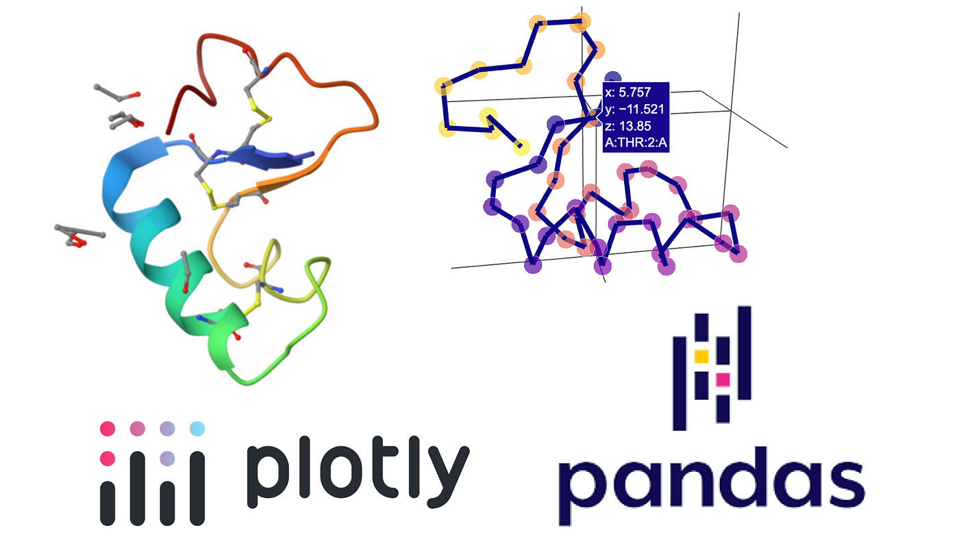
The Graphein package in Python (built using Plotly) can also be used to visualize proteins.

Each residue here is represented and connected by its alpha Carbon.

from graphein.protein.visualisation import plotly_protein_structure_graph

p = plotly_protein_structure_graph(
g,
colour_edges_by="kind",
colour_nodes_by="seq_position",
label_node_ids=False,
plot_title="3NIR Backbone Protein Graph",
node_size_multiplier=1,
)
p.show()

Working with multi-chain PDB files

Let us not limit ourselves to unique protein chains. Proteins often form complexes because many biological processes require the coordinated action of multiple proteins. A multi-chain protein is a protein complex composed of more than one polypeptide chain, each encoded by a separate gene, that interact together to perform a specific function or set of functions.

For this let's take the 6KDE (heterodimer) complex. Looking at the header in the PDB file (download here) we notice we have information about each chain:

HEADER OXIDOREDUCTASE 02-JUL-19 6KDE
TITLE CRYSTAL STRUCTURE OF THE ALPHA BETA HETERODIMER OF HUMAN IDH3 IN
TITLE 2 COMPLEX WITH CA(2+)
COMPND MOL_ID: 1;
COMPND 2 MOLECULE: ISOCITRATE DEHYDROGENASE [NAD] SUBUNIT ALPHA,
COMPND 3 MITOCHONDRIAL;
COMPND 4 CHAIN: A, C;
COMPND 5 SYNONYM: ISOCITRIC DEHYDROGENASE SUBUNIT ALPHA,NAD(+)-SPECIFIC ICDH
COMPND 6 SUBUNIT ALPHA;
COMPND 7 EC: 1.1.1.41;
COMPND 8 ENGINEERED: YES;
COMPND 9 MOL_ID: 2;
COMPND 10 MOLECULE: ISOCITRATE DEHYDROGENASE [NAD] SUBUNIT BETA, MITOCHONDRIAL;
COMPND 11 CHAIN: B, D;
COMPND 12 SYNONYM: ISOCITRIC DEHYDROGENASE SUBUNIT BETA,NAD(+)-SPECIFIC ICDH
COMPND 13 SUBUNIT BETA;
COMPND 14 ENGINEERED: YES

The complex is formed of chains A and C (subunit alpha) binding with chains B and D (subunit beta). Plotting the atomic point cloud colored by chain id gives:

df, df_header = read_pdb_to_dataframe('6kde.pdb')
fig = px.scatter_3d(df, x='x_coord', y='y_coord', z='z_coord', color='chain_id')
fig.update_traces(marker_size = 4)

fig.show()

We can look only at the complex formed by chains A and B. Each atom in the dataframe is linked to a specific chain with the chain_id attribute.

df = pd.concat((df[df['chain_id']=='A'], df[df['chain_id']=='B']))

> > > df['chain_id'].unique()
> > > array(['A', 'B'], dtype=object)

This again highlights how easy it is to manipulate protein data with Pandas. Plotting the updated dataframe df using the same code as above:

Extracting protein interfaces using Pandas

Protein interfaces play a crucial role in understanding the function and interactions of proteins within biological systems. To illustrate working with multi-chain proteins, we can extracting the interface or contact between two chains. The function below shows how this can be achieved easily using numpy.

import numpy as np

def get_contact_atoms(df1: pd.DataFrame, df2:pd.DataFrame = None , threshold:float = 7., coord_names=['x_coord', 'y_coord', 'z_coord']):

# Extract coordinates from dataframes

coords1 = df1[coord_names].to_numpy()
coords2 = df2[coord_names].to_numpy()

    # Compute pairwise distances between atoms
    dist_matrix = np.sqrt(((coords1[:, None] - coords2) ** 2).sum(axis=2))

    # Create a new dataframe containing pairs of atoms whose distance is below the threshold
    pairs = np.argwhere(dist_matrix < threshold)
    atoms1, atoms2 = df1.iloc[pairs[:, 0]], df2.iloc[pairs[:, 1]]
    atoms1_id = atoms1['chain_id'].map(str) + ":" + atoms1['residue_name'].map(str) + ":" + atoms1['residue_number'].map(str)
    atoms2_id = atoms2['chain_id'].map(str) + ":" + atoms2['residue_name'].map(str) + ":" + atoms2['residue_number'].map(str)
    node_pairs = np.vstack((atoms1_id.values, atoms2_id.values)).T
    result = pd.concat([df1.iloc[np.unique(pairs[:, 0])], df2.iloc[np.unique(pairs[:, 1])]])

    return result, node_pairs

In this example we will get all atoms between chains A and B that are 7 Angstrom appart:

df_A = df[df['chain_id']=='A']
df_B = df[df['chain_id']=='B']
contact_atoms, node_pairs = get_contact_atoms(df_A, df_B, 7.)

Plotting this in Plotly, the interface is highlighted in Orange:

import plotly.express as px
import plotly.graph_objects as go

# Create 3D scatter plots for df_A, df_B, and contact_atoms

fig = go.Figure()

# Add trace for df_A

fig.add_trace(
go.Scatter3d(
name='Chain A',
x=df_A['x_coord'],
y=df_A['y_coord'],
z=df_A['z_coord'],
mode='markers',
marker=dict(size=4, color='blue', opacity=0.5), # Adjust opacity here
)
)

# Add trace for df_B

fig.add_trace(
go.Scatter3d(
name='Chain B',
x=df_B['x_coord'],
y=df_B['y_coord'],
z=df_B['z_coord'],
mode='markers',
marker=dict(size=4, color='red', opacity=0.5), # Adjust opacity here
)
)

# Add trace for contact_atoms

fig.add_trace(
go.Scatter3d(
name='Contact Atoms',
x=contact_atoms['x_coord'],
y=contact_atoms['y_coord'],
z=contact_atoms['z_coord'],
mode='markers',
marker=dict(size=6, color='orange'), # You can adjust the color and opacity here
)
)

# Customize the layout

fig.update_layout(
scene=dict(
aspectmode="cube", # To maintain equal axis scaling
),
margin=dict(l=0, r=0, b=0, t=0),
)

# Show the plot

fig.show()

Conclusion

We've explored how to utilize BioPandas and ProDy for loading PDB files into Pandas dataframes, and how to manipulate and visualize protein data using standard Pandas operations. We've also touched on the use of Graphein for constructing protein graphs and Plotly for 3D visualization of protein structures.

Moreover, we've demonstrated how to handle multi-chain PDB files and extract protein interfaces, further expanding the scope of analysis. These techniques open up a wide range of possibilities for protein structure analysis, from studying protein-protein interactions to designing new drugs.

As we've seen, the combination of Python and its scientific libraries offers a flexible and efficient way to handle, analyze, and visualize protein structures.