Fitting numerical data to models is a routine task in all of engineering and science. So you should know your tools and how to use them. In today's article, I give you a short introduction to how you can use Python's scientific working horses NumPy and SciPy to do that. And I will also give some hints on your workflow when fitting data.
A Simple Fit
Suppose we have an array with data from somewhere, and we have to make sense out of it. When we plot it, it may look like that:
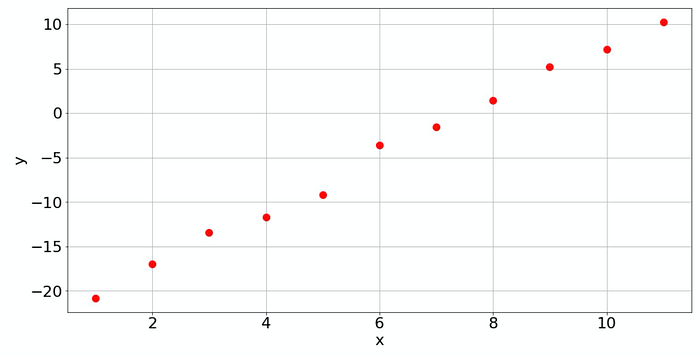
Visually, the human eye recognizes that this is data scattered around a line with a certain slope. So let's fit a line, which is a polynomial of degree 1. If a linear or polynomial fit is all you need, then NumPy is a good way to go. It can easily perform the corresponding least-squares fit:
import numpy as np
x_data = np.arange(1, len(y_data)+1, dtype=float)
coefs = np.polyfit(x_data, y_data, deg=1)
poly = np.poly1d(coefs)
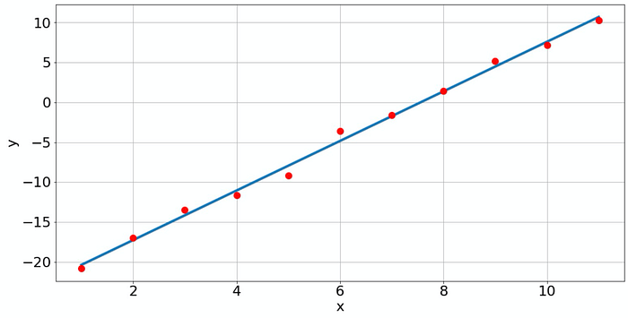
In NumPy, this is a 2-step process. First, you make the fit for a polynomial degree (deg) with np.polyfit. This function returns the coefficients of the fitted polynomial. I'm unable to remember the sorting of the returned coefficients. Is it for the highest degree first or lowest degree first? Instead of looking up the documentation every time, I prefer to use np.poly1d. It automatically creates a polynomial from the coefficients and it surely does remember the sorting. ;-) Then you can use the polynomial just like any normal Python function. Let's plot the fitted line together with the data:
import matplotlib.pyplot as plt
x_model = np.linspace(x_data[0], x_data[-1], 200)
plt.plot(x_model, poly(x_model))
plt.plot(x_data, y_data, 'ro',)
plt.xlabel('x')
plt.ylabel('y')
plt.grid()
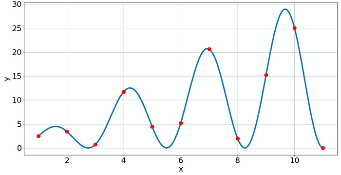
Of course, with np.polyfit we are not restricted to fitting lines, but we can fit a polynomial of any order if enough data points are available. The question is just if it makes sense. For instance, if we fit a polynomial of degree 10 to the data, we get the following result.
coefs = np.polyfit(x_data, y_data, 10)
poly = np.poly1d(coefs)
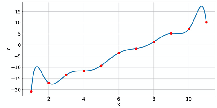
Now the fitted polynomial matches the given data points perfectly but it has some very implausible oscillations. This is a typical example of overfitting. We can always make our model function complicated enough to reproduce the data points very well. However, the price is the loss of predictability. If I want to know the probable value for x=10.5, where no raw data point is given, I would trust the simple model more than the complex model!
Know Your Data!
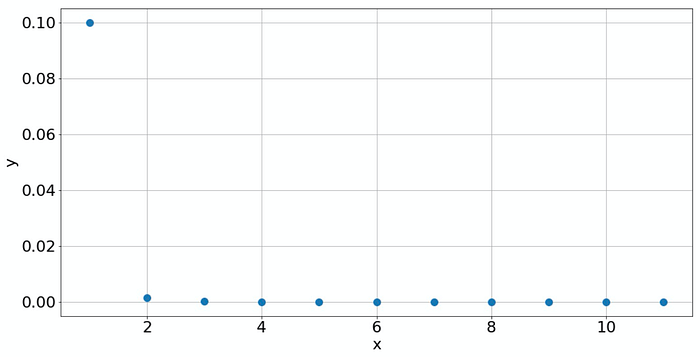
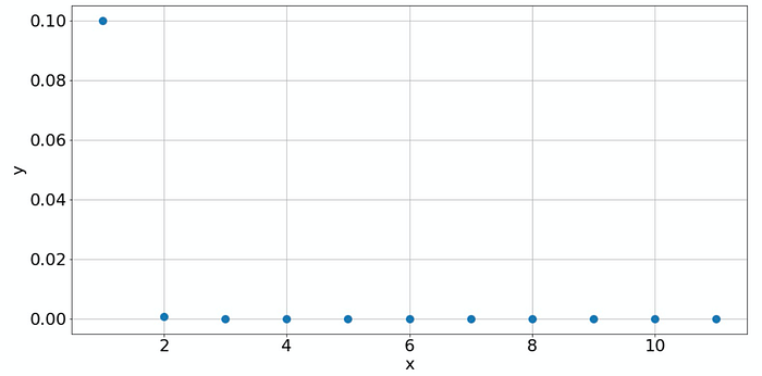
To avoid the effect of overfitting, it is always good to get more knowledge about your data. If you know what process has created your data and if there is a good model for this process (like a physical law), then that is great! But this happens only rarely. But often, you can find out more about your data without making guesses. Plotting your data should always be part of your routine. Consider the following example. If you plot the data in a normal way, then you only see a peak at 𝑥=1and all other values are practically zero. So what should we do? Plot the data on a double-logarithmic scale! This reveals if the data is generated by some power law.
plt.loglog(x_data, y_data, 'o')
plt.grid()
plt.xlabel('x')
plt.ylabel('y')
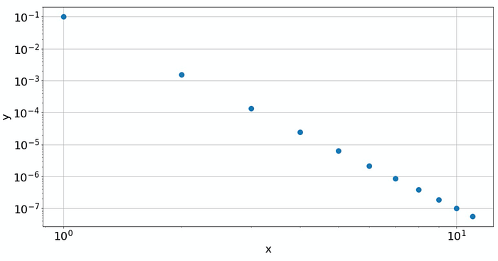
A double-logarithmic plot reveals that the data is based on a power law
The double-log plot shows a linear behavior, which means that the data is from a power law. And the slope of the line gives the power itself. Increasing 𝑥 by a factor of 10 reduces 𝑦 by a factor of 10⁶. So, we have a power law
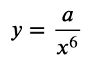
for some constant 𝑎. If you don't want to read off the magnitudes, then just plot it on the log-log scale to see if the behavior is a power law, and then fit the log-log data to a line:
coefs = np.polyfit(np.log(x_data), np.log(y_data), deg=1)
coefs
Out: array([-6.        , -2.30258509])
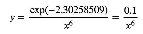
So here, we see immediately that the power is -6. What we have is:

or taking the exponential:
Let's see some other examples. Suppose we have the following data:
Looks almost the same as before, right? But not so, if you plot it on the log-log scale:
plt.loglog(x_data, y_data, 'o')
plt.xlabel('x')
plt.ylabel('y')
plt.grid()
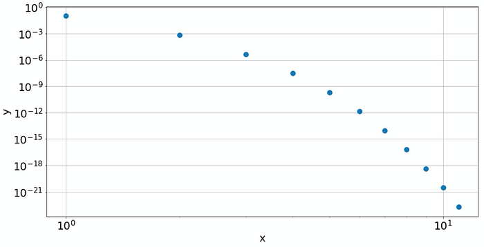
The double-logarithmic plot shows that this is not a power law
Now the log-log plot is not a straight line anymore. This indicates that we don't have a power law. Instead, with increasing 𝑥, the values for 𝑦 decrease faster than any power. Probably it's something that contains an exponential. If it is exponential, this should be visible in a semi-logarithmic plot:
plt.semilogy(x_data, y_data, 'o')
plt.xlabel('x')
plt.ylabel('y')
plt.grid()
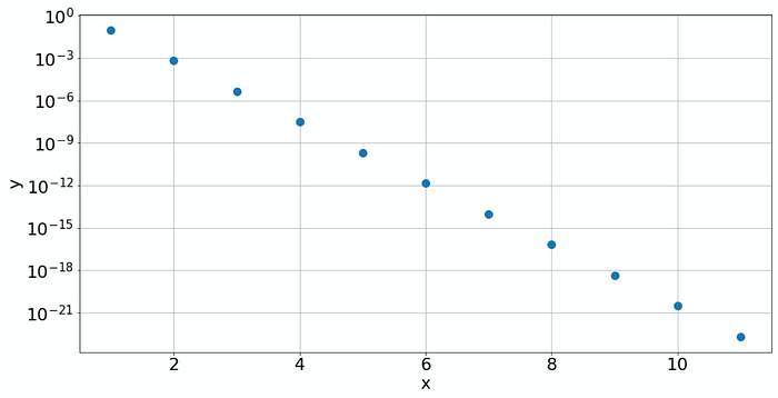
The semilog plot reveals that the law is an exponential
Yes, clearly a line, so our data must have been created by law:
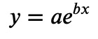
with constants 𝑎 and 𝑏. We can get the constants with NumPy again:
coefs = np.polyfit(x_data, np.log(y_data), deg=1)
coefs
Out: array([-5.        ,  2.69741491])
The slope in the semilog plot corresponds to the constant 𝑏, and the offset of the fit encodes the constant 𝑎:
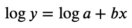
So 𝑏=−5 and 𝑎=exp(2.69741491)=14.8413.
Fitting nonlinear models with SciPy
NumPy's polyfit function can only fit polynomials of a given degree. So if your data was generated by a process with some law:
it will not work. In that situation, you can use SciPy instead. Here you, can define a given law and tell SciPy to optimize the parameters. Consider the following example:
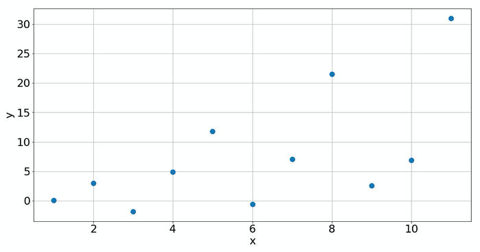
Just from the plot, it's difficult to judge what law is behind that data. But if you do know the law (for instance you know the physical process involved), then you can easily model it with scipy.optimize.curve_fit. Here, we assume that the law is the one given above.
from scipy.optimize import curve_fit
def law(x, a, b):
    return a * x * np.sin(x)**2 + b
fit = curve_fit(law, x_data, y_data)
fit
Out: (array([ 3., -2.]),
      array([[ 5.49796736e-32, -1.80526189e-31],
        [-1.80526189e-31,  1.16149599e-30]]))
The output is a tuple of two arrays. The first array contains the fitted parameters, the second array gives information on how good the fit is. In our case, since we know the exact law and the data is not noisy, we get a perfect fit.
y_model = law(x_model, *fit[0])
plt.plot(x_model, y_model)
plt.plot(x_data, y_data, 'ro')
plt.grid()
plt.xlabel('x')
plt.ylabel('y')
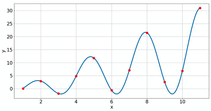
The oscillations here are not overfitting because we assumed that we know the law behind the data, so that's ok.
Finally, let's have a look at a still more complicated situation. Up to now, all fitting that was done was linear fitting. That does not mean that the curves are linear, but the parameters of the fit appeared only with powers of 1. This is not the case anymore if you want to fit data to a law like
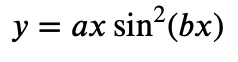
Note that now the parameter 𝑏 is inside the sine function. And if you write the sine function as a power series, you see that 𝑏 not only appears with the power of 1 but with infinitely many other powers. This is now called nonlinear fitting, and it can be an art to get a good solution. There is no fits-all-purpose guideline and what you should do, depends very much on the problem. In our case we get:
def law(x, a, b):
    return a * x * np.sin(b*x)**2
fit = curve_fit(law, x_data, y_data)
fit
Out: (array([3.        , 1.14159265]),
      array([[1.69853790e-30, 1.08926835e-32],
        [1.08926835e-32, 2.07061942e-33]]))
Although the fit looks good again, it contains some errors not visible in the plot and also not in the confidence output. Since I created the data manually, I know that the fitted value for 𝑎 is fine, but for 𝑏 it is off (1.14159 instead of 2). So what can you do to judge if your fit is good? Don't use all data for the fitting! Reserve some data, and only do the fit with the rest of the data. Then use the reserved data to check if the fit predicts the unseen data. That's called train-test-split.
Often, non-linear fits need some help from the user. For instance, you may want to give initial guesses for the parameters manually, or you want to bound or constrain parameters to certain ranges or conditions. That can all be done with the additional arguments of curve_fit. But that's a big topic suitable for a complete post, so I save it for some later time. Stay tuned. :-)
Comments
Loading comments…