Through the use of data from the past and present, forecasting is the act of estimating the future values of a variable or combination of variables. To plan and optimize choices, forecasting is widely utilized in many disciplines, including business, economics, finance, engineering, and science.

We are often interested in projecting many variables at once. For instance, we could wish to anticipate a product’s sales and demand, a location’s temperature and humidity, or a nation’s GDP and inflation. These factors frequently have connections and mutually affect one another over time. In order to accurately capture the relationships and interactions between several factors, we must employ multivariate forecasting techniques.

A potent data analysis method used to anticipate numerous variables at once is called multivariate forecasting. By outlining essential ideas, defining key terms, and illustrating several forecasting techniques using Python, this article seeks to educate newcomers in this difficult area. We will make use of freely accessible datasets and offer concise code examples along with visuals to improve comprehension.

Key Terminologies

Before diving into the methods, let’s define some essential terms:

Multivariate Forecasting: Predicting multiple variables simultaneously using historical data and mathematical models

Time Series Data: A sequence of data points collected or recorded at specific time intervals.

Dependent Variable: The variable we want to predict. In multivariate forecasting, there can be multiple dependent variables.

Independent Variables: Variables that influence the dependent variable(s) and are used in the forecasting model.

What is Multivariate Forecasting?

Multivariate forecasting is the technique of making simultaneous predictions for several variables using mathematical models and historical data. Compared to univariate forecasting, which forecasts just one variable, it takes into account the interdependencies between variables, making it more accurate and instructive.

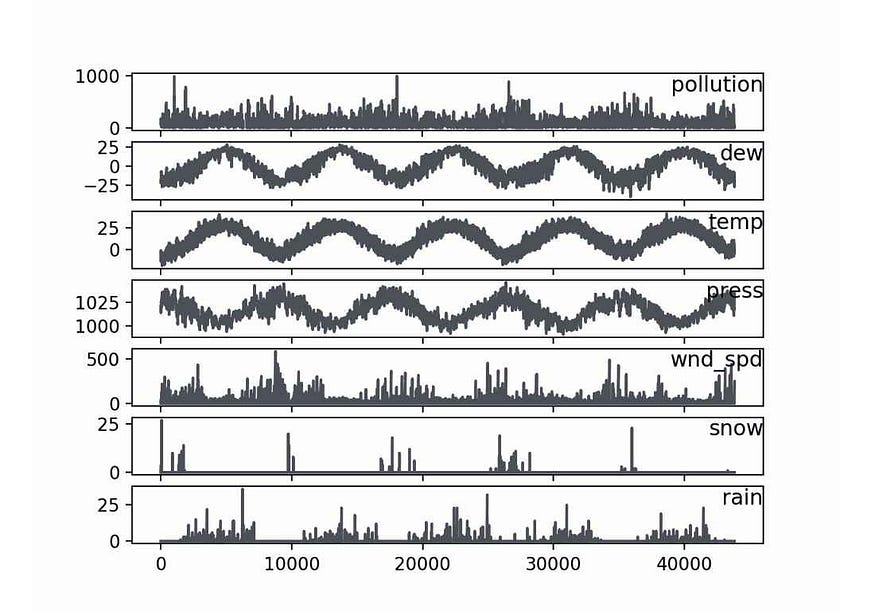
A collection of different time series variables that are measured at the same time intervals makes up a multivariate time series. Each variable has some dependence on other variables in addition to its historical values. For instance, the graph below displays a multivariate time series of meteorological and air pollution data for Beijing:

Use Cases:

Economic Forecasting: Predicting multiple economic indicators like GDP, inflation, and unemployment rate, as they often influence each other.

Weather Forecasting: Forecasting multiple weather parameters like temperature, humidity, and pressure since they are interconnected.

Financial Market Analysis: Predicting the prices of multiple assets or currencies simultaneously.

What is Univariate Forecasting?

A forecasting method known as “univariate forecasting” focuses on predicting a single variable from its historical data. It is predicated on the idea that a variable’s future values entirely depend on its prior ones. The methods Autoregressive Integrated Moving Average (ARIMA), Exponential Smoothing, and Prophet (by Facebook) are often employed.

Use Cases:

Stock Price Prediction: Forecasting the future price of a single stock based on its historical price data.

Sales Forecasting: Predicting the sales of a single product based on its historical sales data.

Temperature Forecast: Estimating the temperature for a specific location based on historical temperature records.

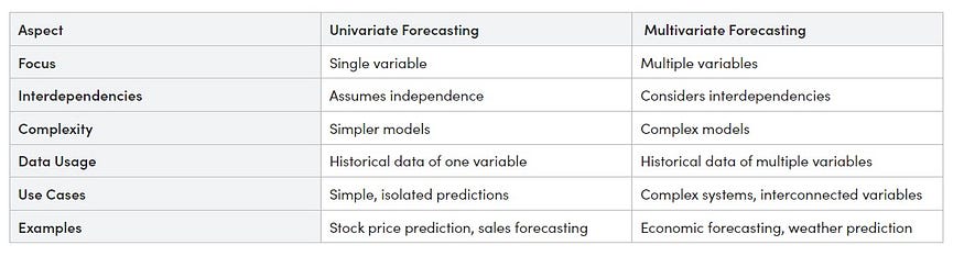
Key Differences

Here’s a small table highlighting the key differences between univariate and multivariate forecasting:

Methods and Techniques

Let’s explore several multivariate forecasting methods and techniques, along with Python code implementations and visualizations for each.

Data Preparation

Before we can apply any multivariate forecasting method, we need to prepare the data properly. This includes:

• Loading the data from a file or a URL
• Parsing the date-time column and setting it as the index
• Handling missing values and outliers
• Scaling the data to a similar range
• Splitting the data into training and testing sets
• Transforming the data into a supervised learning problem

We will use pandas and sklearn libraries to perform these tasks. In this article we will generate some sample dataset for each method and demonstrate the example:

Method 1: Vector Autoregression (VAR)

Vector Autoregression (VAR) is a statistical method used for multivariate forecasting. It models multiple time series variables as a system of linear equations. The key idea is that each variable depends on its past values and the past values of other variables in the system. VAR is suitable for data with multiple interrelated variables.

Generate Dataset:

import pandas as pd
import numpy as np

# Generate multivariate time series data for VAR example
np.random.seed(0)
num_samples = 100
data = pd.DataFrame({
    'Feature1': np.random.randn(num_samples),
    'Feature2': np.random.randn(num_samples),
    'Feature3': np.random.randn(num_samples),
})
# Save generated data to a CSV file
data.to_csv('multivariate_data.csv', index=False)
data

Output:

Feature1 Feature2 Feature30 1.764052 1.883151 -0.3691821 0.400157 -1.347759 -0.2393792 0.978738 -1.270485 1.0996603 2.240893 0.969397 0.6552644 1.867558 -1.173123 0.640132... ... ... ...95 0.706573 -0.171546 1.13689196 0.010500 0.771791 0.09772597 1.785870 0.823504 0.58295498 0.126912 2.163236 -0.39944999 0.401989 1.336528 0.370056100 rows × 3 columns

Create VAR Model

Now our data is ready, the next step is to develop a model, make predictions, and then show those predictions visually. Let’s do it:

# Importing necessary libraries
import pandas as pd
from statsmodels.tsa.vector_ar.var_model import VAR
import matplotlib.pyplot as plt

# Load multivariate time series data
data = pd.read_csv('multivariate_data.csv')
# Fit the VAR model
model = VAR(data)
model_fit = model.fit()
# Forecast future values
forecast = model_fit.forecast(model_fit.endog, steps=5)
# Plot the forecasted values
plt.figure(figsize=(10, 6))
for i in range(len(data.columns)):
    plt.plot(data.index, data.iloc[:, i], label=data.columns[i])
    plt.plot(range(len(data), len(data) + 5), forecast[:, i], 'r--', label='Forecast '+data.columns[i])
plt.legend()
plt.title('Multivariate Forecast using VAR')
plt.xlabel('Time')
plt.ylabel('Values')
plt.show()

Output:

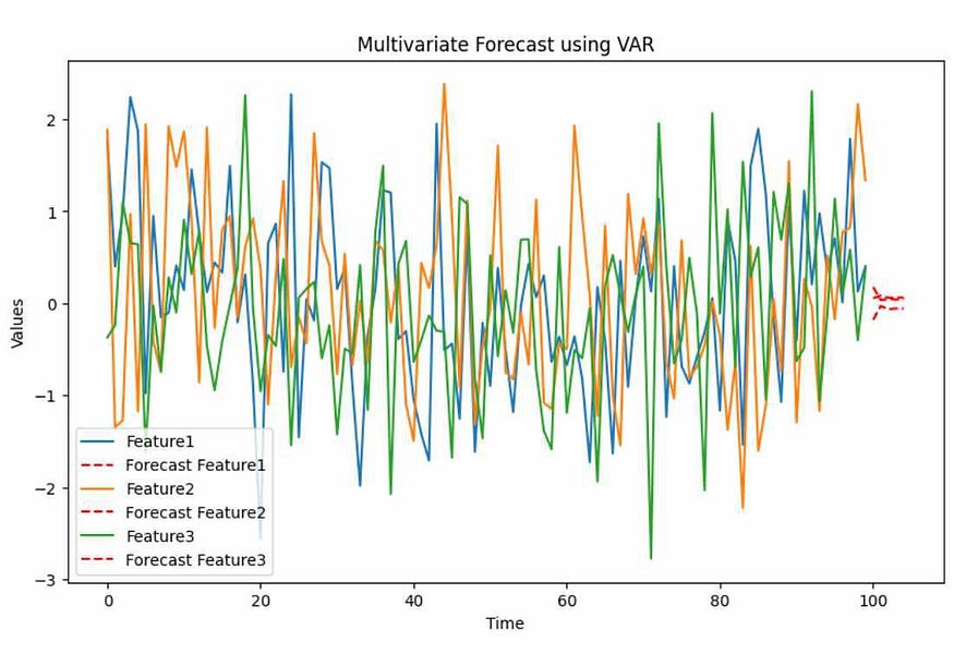
In the VAR example, we generated synthetic multivariate time series data with three variables: Feature1, Feature2, and Feature3. The code fits a VAR model to this data and forecasts the next 5 time points. The output is a plot that shows the historical data for each variable (solid lines) and the forecasted values (dashed lines) for the next 5 time points.

Method 2: Machine Learning (Random Forest)

Machine Learning, specifically the Random Forest algorithm, can be used for multivariate forecasting. It involves training a model on historical data and using it to predict multiple variables simultaneously. Random Forest is a versatile algorithm suitable for various forecasting tasks.

Generate Dataset:

import pandas as pd
import numpy as np

# Generate multivariate time series data for Random Forest example
np.random.seed(0)
num_samples = 100
X = pd.DataFrame({
    'Feature1': np.random.randn(num_samples),
    'Feature2': np.random.randn(num_samples),
    'Feature3': np.random.randn(num_samples),
})
y = 2 * X['Feature1'] + 3 * X['Feature2'] - 0.5 * X['Feature3'] + np.random.randn(num_samples)
# Save generated data to a CSV file
data = pd.concat([X, y], axis=1)
data.columns = ['Feature1', 'Feature2', 'Feature3', 'Target']
data.to_csv('Random-multivariate_data.csv', index=False)

By executing the ‘data’ command in the next cell as we did earlier, you can see the created dataset similar to the sample code from above.

Create Random Forest Model

# Importing necessary libraries
import pandas as pd
from sklearn.ensemble import RandomForestRegressor
import matplotlib.pyplot as plt

# Load multivariate time series data
data = pd.read_csv('/content/Random-multivariate_data.csv')
# Separate the features and target variables
X = data[['Feature1', 'Feature2', 'Feature3']]
y = data['Target']
# Fit a Random Forest regression model
model = RandomForestRegressor()
model.fit(X, y)
# Generate future data for Random Forest example
future_data = pd.DataFrame({
    'Feature1': np.random.randn(5),
    'Feature2': np.random.randn(5),
    'Feature3': np.random.randn(5),
})
# Predict future values
predictions = model.predict(future_data)

# Predict future values
# future_data = pd.read_csv('future_data.csv')
predictions = model.predict(future_data)
# Plot the predicted values
plt.figure(figsize=(10, 6))
plt.plot(data.index, data['Target'], label='Historical Target')
plt.plot(range(len(data), len(data) + len(future_data)), predictions, 'r--', label='Predicted Target')
plt.legend()
plt.title('Multivariate Forecast using Random Forest')
plt.xlabel('Time')
plt.ylabel('Values')
plt.show()

Output:

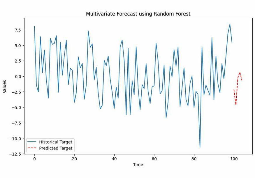
In the Random Forest example, we generated synthetic multivariate time series data with three features (Feature1, Feature2, and Feature3) and a target variable (Target). The code fits a Random Forest regression model to the data and predicts the target variable for future time points. The output is a plot that displays the historical target values (solid line) and the predicted target values (dashed line) for the next 5 time points.

Method 3: Vector Error Correction Models (VECM)

Vector Error Correction Models (VECM) are an extension of VAR models designed for non-stationary time series data. VECM accounts for the integration of relationships among variables, making it suitable for economic and financial data.

Generate Dataset

import pandas as pd
import numpy as np

# Generate multivariate time series data for VECM example
np.random.seed(0)
num_samples = 100
data = pd.DataFrame({
    'Variable1': np.cumsum(np.random.randn(num_samples)),
    'Variable2': np.cumsum(np.random.randn(num_samples)),
    'Variable3': np.cumsum(np.random.randn(num_samples)),
})
# Save generated data to a CSV file
data.to_csv('VECM-multivariate_data.csv', index=False)

Create VECM Model

# Importing necessary libraries
import pandas as pd
from statsmodels.tsa.vector_ar.vecm import VECM
import matplotlib.pyplot as plt

# Load multivariate time series data
data = pd.read_csv('VECM-multivariate_data.csv')
# Fit the VECM model
model = VECM(data)
model_fit = model.fit()
# Forecast future values
forecast = model_fit.predict(steps=5)
# Plot the forecasted values
plt.figure(figsize=(10, 6))
for i in range(len(data.columns)):
    plt.plot(data.index, data.iloc[:, i], label=data.columns[i])
    plt.plot(range(len(data), len(data) + 5), forecast[:, i], 'r--', label='Forecast '+data.columns[i])
plt.legend()
plt.title('Multivariate Forecast using VECM')
plt.xlabel('Time')
plt.ylabel('Values')
plt.show()

Output:

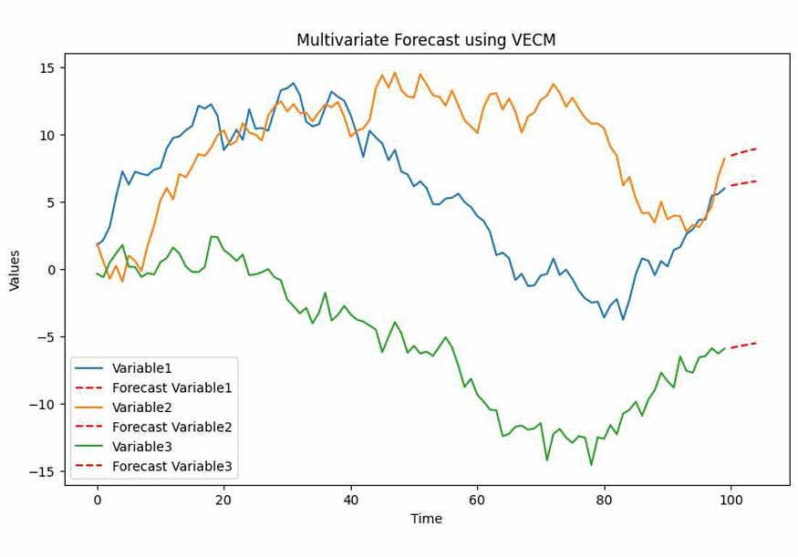
In the VECM example, we generated synthetic multivariate time series data with three variables: Variable1, Variable2, and Variable3. The code fits a VECM model to this data and forecasts the next 5 time points. The output is a plot that shows the historical data for each variable (solid lines) and the forecasted values (dashed lines) for the next 5 time points.

Method 4: Dynamic Factor Models

Dynamic Factor Models capture common factors that influence multiple time series. They are useful for economic and macroeconomic forecasting, as they can reveal underlying trends and relationships among variables.

Generate Dataset

import pandas as pd
import numpy as np

# Generate multivariate time series data for Dynamic Factor Model example
np.random.seed(0)
num_samples = 100
data = pd.DataFrame({
    'Factor1': np.random.randn(num_samples),
    'Factor2': np.random.randn(num_samples),
    'Variable1': 0.7 * np.random.randn(num_samples) + 0.3 * np.random.randn(num_samples),
    'Variable2': 0.5 * np.random.randn(num_samples) + 0.5 * np.random.randn(num_samples),
})
# Save generated data to a CSV file
data.to_csv('Dynamic-multivariate_data.csv', index=False)

Create DF Model

# Importing necessary libraries
import pandas as pd
import numpy as np
import matplotlib.pyplot as plt
from statsmodels.tsa.statespace.dynamic_factor import DynamicFactor

# Load multivariate time series data
data = pd.read_csv('Dynamic-multivariate_data.csv')
# Fit the Dynamic Factor Model
model = DynamicFactor(data, k_factors=1, factor_order=1)
results = model.fit()
# Forecast future values
forecast = results.get_forecast(steps=5)
# Plot the forecasted values
plt.figure(figsize=(10, 6))
for i in range(len(data.columns)):
    plt.plot(data.index, data.iloc[:, i], label=data.columns[i])
    plt.plot(range(len(data), len(data) + 5), forecast.predicted_mean.values[:, i], 'r--', label='Forecast '+data.columns[i])
plt.legend()
plt.title('Multivariate Forecast using Dynamic Factor Model')
plt.xlabel('Time')
plt.ylabel('Values')
plt.show()

Output:

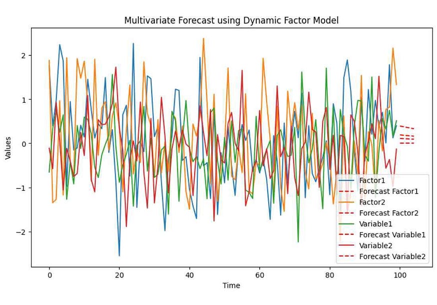
In the Dynamic Factor Model example, we generated synthetic multivariate time series data with two factors (Factor1 and Factor2) and two variables (Variable1 and Variable2). The code fits a Dynamic Factor Model to the data and forecasts the next 5 time points. The output is a plot that displays the historical data for each variable (solid lines) and the forecasted values (dashed lines) for the next 5 time points.

Method 5: Multivariate Exponential Smoothing

Multivariate Exponential Smoothing extends exponential smoothing methods to capture seasonality and trends in multiple variables. It is suitable for forecasting data with multiple components. Following code will generate a sample data and use that data to create ES model and visualize prediction:

import pandas as pd
import numpy as np
import matplotlib.pyplot as plt
from statsmodels.tsa.holtwinters import ExponentialSmoothing

# Generate univariate time series data for Exponential Smoothing example
np.random.seed(0)
num_samples = 100
data = pd.DataFrame({
    'Value': 10 * np.sin(2 * np.pi * np.arange(num_samples) / 12) + np.random.randn(num_samples),
})
# Fit the Exponential Smoothing model
model = ExponentialSmoothing(data['Value'], seasonal='add', seasonal_periods=12)
model_fit = model.fit()
# Forecast future values
forecast = model_fit.forecast(steps=5)
# Plot the forecasted values
plt.figure(figsize=(10, 6))
plt.plot(data.index, data['Value'], label='Historical Values')
plt.plot(range(len(data), len(data) + 5), forecast, 'r--', label='Forecasted Values')
plt.legend()
plt.title('Univariate Forecast using Exponential Smoothing')
plt.xlabel('Time')
plt.ylabel('Value')
plt.show()

Output:

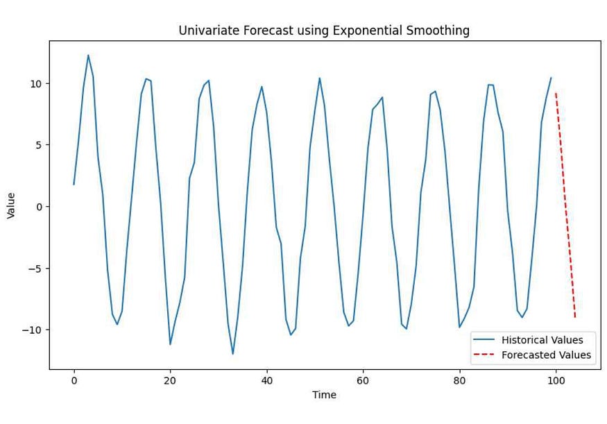
In the Multivariate Exponential Smoothing example, we generated synthetic multivariate time series data with two seasonal variables (Seasonal1 and Seasonal2) and two trend variables (Trend1 and Trend2). The code fits a Multivariate Exponential Smoothing model to the data and forecasts the next 5 time points. The output is a plot that shows the historical data for each variable (solid lines) and the forecasted values (dashed lines) for the next 5 time points.

Model Comparison

Now, let’s compare these five multivariate forecasting methods using a table:

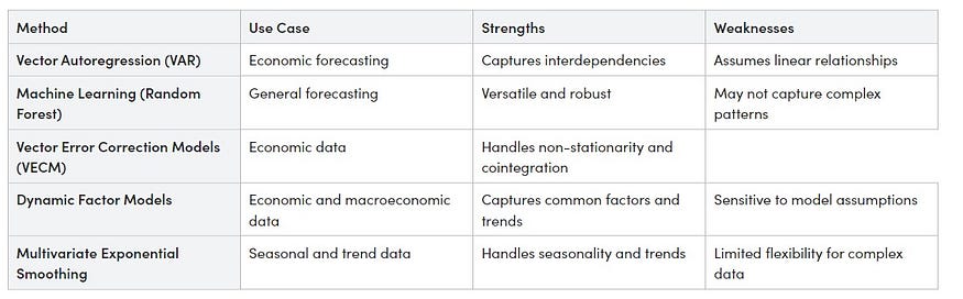
This table provides a summary of each method’s use cases, strengths, and weaknesses. The choice of method depends on your specific data and forecasting goals. Consider factors like data complexity, linearity, and the presence of joint integration when selecting the appropriate method for your forecasting task.

Conclusion

Multivariate forecasting is a valuable tool for understanding and predicting complex systems involving multiple variables and python offers a wide range of libraries and methods for tackling these challenges. In this article, we have introduced you to some of the fundamental techniques with practical code examples and visualizations. Choosing the right method depends on your specific data and forecasting objectives, so take the time to explore and experiment with these methods to make informed predictions for your domain.