Denoising Autoencoder in Pytorch on MNIST Dataset

Image made by Author

The post is the eighth in a series of guides to building deep learning models with Pytorch. Below, there is the full series:

1. Pytorch Tutorial for Beginners
2. Manipulating Pytorch Datasets
3. Understand Tensor Dimensions in DL models
4. CNN & Feature visualizations
5. Hyperparameter tuning with Optuna
6. K Fold Cross Validation
7. Convolutional Autoencoder
8. Denoising Autoencoder (this post)
9. Variational Autoencoder

The goal of the series is to make Pytorch more intuitive and accessible as possible through examples of implementations. There are many tutorials on the Internet to use Pytorch to build many types of challenging models, but it can also be confusing at the same time because there are always slight differences when you pass from one tutorial to another. In this series, I want to start from the simplest topics to the more advanced ones.

Denoising Autoencoder

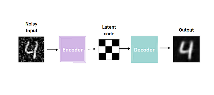
The Denoising Autoencoder is an extension of the autoencoder. Just like a standard autoencoder, it's composed of an encoder, that compresses the data into the latent code, extracting the most relevant features, and a decoder, which decompress it and reconstructs the original input. There is only a slight modification: the Denoising Autoencoder takes a noisy image as input and the target for the output layer is the original input without noise.

This type of encoder is useful for many reasons. First, it reduces the risk of overfitting and prevents the autoencoder from learning a simple identity function. Moreover, the encoded space of the autoencoder contains more robust information that allows the reconstruction of images. In other words, the noise added to the input act as a regularizer. In this tutorial, the technique considered to corrupt the images is called Gaussian Noise.

Implementation with Pytorch

The Denoising autoencoder is applied to the MNIST dataset, as in most of the previous posts of the series.

Let's import the libraries and the dataset:

import matplotlib.pyplot as plt # plotting library
import numpy as np # this module is useful to work with numerical arrays
import pandas as pd
import random
import torch
import torchvision
from torchvision import transforms
from torch.utils.data import DataLoader,random_split
from torch import nn
import torch.nn.functional as F
import torch.optim as optim

data_dir = 'dataset'

train_dataset = torchvision.datasets.MNIST(data_dir, train=True, download=True)
test_dataset = torchvision.datasets.MNIST(data_dir, train=False, download=True)

train_transform = transforms.Compose([
transforms.ToTensor(),
])

test_transform = transforms.Compose([
transforms.ToTensor(),
])

train_dataset.transform = train_transform
test_dataset.transform = test_transform

m=len(train_dataset)

train_data, val_data = random_split(train_dataset, [int(m-m*0.2), int(m*0.2)])
batch_size=256

train_loader = torch.utils.data.DataLoader(train_data, batch_size=batch_size)
valid_loader = torch.utils.data.DataLoader(val_data, batch_size=batch_size)
test_loader = torch.utils.data.DataLoader(test_dataset, batch_size=batch_size,shuffle=True)

Now, it's time to define the encoder and the decoder classes, which both contain 3 convolutional layers and 2 fully connected layers.

class Encoder(nn.Module):

	def __init__(self, encoded_space_dim,fc2_input_dim):
		super().__init__()

		### Convolutional section
		self.encoder_cnn = nn.Sequential(
		nn.Conv2d(1, 8, 3, stride=2, padding=1),
		nn.ReLU(True),
		nn.Conv2d(8, 16, 3, stride=2, padding=1),
		nn.BatchNorm2d(16),
		nn.ReLU(True),
		nn.Conv2d(16, 32, 3, stride=2, padding=0),
		nn.ReLU(True)
		)

		### Flatten layer
		self.flatten = nn.Flatten(start_dim=1)
### Linear section
		self.encoder_lin = nn.Sequential(
			nn.Linear(3 * 3 * 32, 128),
			nn.ReLU(True),
			nn.Linear(128, encoded_space_dim)
		)

	def forward(self, x):
		x = self.encoder_cnn(x)
		x = self.flatten(x)
		x = self.encoder_lin(x)
		return x
class Decoder(nn.Module):

	def __init__(self, encoded_space_dim,fc2_input_dim):
		super().__init__()
		self.decoder_lin = nn.Sequential(
			nn.Linear(encoded_space_dim, 128),
			nn.ReLU(True),
			nn.Linear(128, 3 * 3 * 32),
			nn.ReLU(True)
		)

		self.unflatten = nn.Unflatten(dim=1,
		unflattened_size=(32, 3, 3))

		self.decoder_conv = nn.Sequential(
			nn.ConvTranspose2d(32, 16, 3,
			stride=2, output_padding=0),
			nn.BatchNorm2d(16),
			nn.ReLU(True),
			nn.ConvTranspose2d(16, 8, 3, stride=2,
			padding=1, output_padding=1),
			nn.BatchNorm2d(8),
			nn.ReLU(True),
			nn.ConvTranspose2d(8, 1, 3, stride=2,
			padding=1, output_padding=1)
		)

	def forward(self, x):
		x = self.decoder_lin(x)
		x = self.unflatten(x)
		x = self.decoder_conv(x)
		x = torch.sigmoid(x)
		return x

After, we can initialize the encoder and decoder objects, the loss, the optimizer, and the device to use CUDA in the deep learning model.

### Define the loss function
loss_fn = torch.nn.MSELoss()

### Define an optimizer (both for the encoder and the decoder!)
lr= 0.001

### Set the random seed for reproducible results
torch.manual_seed(0)

### Initialize the two networks
d = 4

#model = Autoencoder(encoded_space_dim=encoded_space_dim)
encoder = Encoder(encoded_space_dim=d,fc2_input_dim=128)
decoder = Decoder(encoded_space_dim=d,fc2_input_dim=128)
params_to_optimize = [
	{'params': encoder.parameters()},
	{'params': decoder.parameters()}
]

optim = torch.optim.Adam(params_to_optimize, lr=lr, weight_decay=1e-05)

# Check if the GPU is available
device = torch.device("cuda") if torch.cuda.is_available() else torch.device("cpu")
print(f'Selected device: {device}')

# Move both the encoder and the decoder to the selected device
encoder.to(device)
decoder.to(device)

Finally, I show the most fundamental part, in which I pass the noisy image to the model. Before the training, a function is defined to add noise to the image.

def add_noise(inputs,noise_factor=0.3):
	noisy = inputs+torch.randn_like(inputs) * noise_factor
	noisy = torch.clip(noisy,0.,1.)
	return noisy

There are two steps to transform the image:

• torch.randn_like to create a noisy tensor of the same size of the input
• torch.clip(min=0.,max=1.) to limit the range between 0 and 1

I defined two distinct functions for training and evaluating the model:

### Training function
def train_epoch_den(encoder, decoder, device, dataloader, loss_fn, optimizer,noise_factor=0.3):
	# Set train mode for both the encoder and the decoder
	encoder.train()
	decoder.train()
	train_loss = []
	# Iterate the dataloader (we do not need the label values, this is unsupervised learning)
	for image_batch, _ in dataloader: # with "_" we just ignore the labels (the second element of the dataloader tuple)
		# Move tensor to the proper device
		image_noisy = add_noise(image_batch,noise_factor)
		image_batch = image_batch.to(device)
		image_noisy = image_noisy.to(device)
		# Encode data
		encoded_data = encoder(image_noisy)
		# Decode data
		decoded_data = decoder(encoded_data)
		# Evaluate loss
		loss = loss_fn(decoded_data, image_batch)
		# Backward pass
		optimizer.zero_grad()
		loss.backward()
		optimizer.step()
		# Print batch loss
		print('\t partial train loss (single batch): %f' % (loss.data))
		train_loss.append(loss.detach().cpu().numpy())

	return np.mean(train_loss)

### Testing function
def test_epoch_den(encoder, decoder, device, dataloader, loss_fn,noise_factor=0.3):
	# Set evaluation mode for encoder and decoder
	encoder.eval()
	decoder.eval()
	with torch.no_grad(): # No need to track the gradients
		# Define the lists to store the outputs for each batch
		conc_out = []
		conc_label = []
		for image_batch, _ in dataloader:
			# Move tensor to the proper device
			image_noisy = add_noise(image_batch,noise_factor)
			image_noisy = image_noisy.to(device)
			# Encode data
			encoded_data = encoder(image_noisy)
			# Decode data
			decoded_data = decoder(encoded_data)
			# Append the network output and the original image to the lists
			conc_out.append(decoded_data.cpu())
			conc_label.append(image_batch.cpu())
		# Create a single tensor with all the values in the lists
		conc_out = torch.cat(conc_out)
		conc_label = torch.cat(conc_label)
		# Evaluate global loss
		val_loss = loss_fn(conc_out, conc_label)
	return val_loss.data

We also want to see how the denoising autoencoder is learning to reconstruct the images in each epoch. It's possible by visualizing the original input, the noisy input, and the reconstructed image.

def plot_ae_outputs_den(encoder,decoder,n=10,noise_factor=0.3):
	plt.figure(figsize=(16,4.5))
	targets = test_dataset.targets.numpy()
	t_idx = {i:np.where(targets==i)[0][0] for i in range(n)}
	for i in range(n):

		ax = plt.subplot(3,n,i+1)
		img = test_dataset[t_idx[i]][0].unsqueeze(0)
		image_noisy = add_noise(img,noise_factor)
		image_noisy = image_noisy.to(device)

		encoder.eval()
		decoder.eval()

		with torch.no_grad():
			rec_img = decoder(encoder(image_noisy))

		plt.imshow(img.cpu().squeeze().numpy(), cmap='gist_gray')
		ax.get_xaxis().set_visible(False)
		ax.get_yaxis().set_visible(False)
		if i == n//2:
			ax.set_title('Original images')
		ax = plt.subplot(3, n, i + 1 + n)
		plt.imshow(image_noisy.cpu().squeeze().numpy(), cmap='gist_gray')
		ax.get_xaxis().set_visible(False)
		ax.get_yaxis().set_visible(False)
		if i == n//2:
			ax.set_title('Corrupted images')

		ax = plt.subplot(3, n, i + 1 + n + n)
		plt.imshow(rec_img.cpu().squeeze().numpy(), cmap='gist_gray')
		ax.get_xaxis().set_visible(False)
		ax.get_yaxis().set_visible(False)
		if i == n//2:
			ax.set_title('Reconstructed images')
	plt.subplots_adjust(left=0.1,
					bottom=0.1,
					right=0.7,
					top=0.9,
					wspace=0.3,
					hspace=0.3)
	plt.show()

Now, it's time to train and evaluate the autoencoder using the functions defined before:

### Training cycle
noise_factor = 0.3
num_epochs = 30
history_da={'train_loss':[],'val_loss':[]}

for epoch in range(num_epochs):
	print('EPOCH %d/%d' % (epoch + 1, num_epochs))
	### Training (use the training function)
	train_loss=train_epoch_den(
		encoder=encoder,
		decoder=decoder,
		device=device,
		dataloader=train_loader,
		loss_fn=loss_fn,
		optimizer=optim,noise_factor=noise_factor)
	### Validation (use the testing function)
	val_loss = test_epoch_den(
		encoder=encoder,
		decoder=decoder,
		device=device,
		dataloader=valid_loader,
		loss_fn=loss_fn,noise_factor=noise_factor)
	# Print Validationloss
	history_da['train_loss'].append(train_loss)
	history_da['val_loss'].append(val_loss)
	print('\n EPOCH {}/{} \t train loss {:.3f} \t val loss {:.3f}'.format(epoch + 1, num_epochs,train_loss,val_loss))
	plot_ae_outputs_den(encoder,decoder,noise_factor=noise_factor)

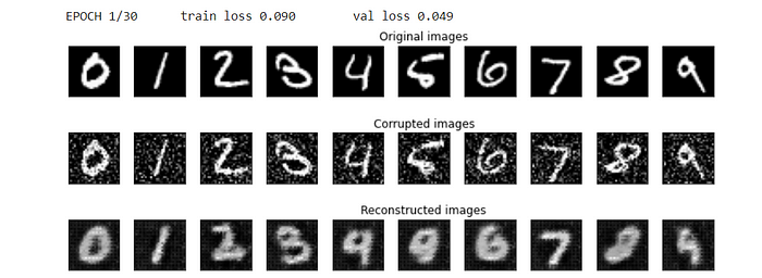
Results in the first epoch

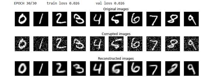
Results after 30 epochs

After 30 epochs, the denoising autoencoder seems to reconstruct similar images to the ones observed in the input. There are still some imperfections, but it's still an improvement with respect to the first epochs, in which the autoencoder didn't still capture the most relevant information to build the reconstructions.

Another way to evaluate the performance of the denoising autoencoder is through the generation of new images from the random latent code.

def show_image(img):
	npimg = img.numpy()
	plt.imshow(np.transpose(npimg, (1, 2, 0)))

encoder.eval()
decoder.eval()

with torch.no_grad():
	# calculate mean and std of latent code, generated takining in test images as inputs
	images, labels = iter(test_loader).next()
	images = images.to(device)
	latent = encoder(images)
	latent = latent.cpu()

	mean = latent.mean(dim=0)
	print(mean)
	std = (latent - mean).pow(2).mean(dim=0).sqrt()
	print(std)

	# sample latent vectors from the normal distribution
	latent = torch.randn(128, d)*std + mean

	# reconstruct images from the random latent vectors
	latent = latent.to(device)
	img_recon = decoder(latent)
	img_recon = img_recon.cpu()

	fig, ax = plt.subplots(figsize=(20, 8.5))
	show_image(torchvision.utils.make_grid(img_recon[:100],10,5))
	plt.show()

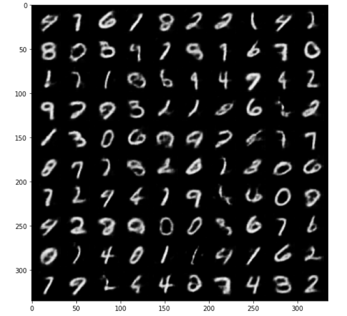
Some digits seem well reconstructed, such as the ones corresponding to 4 and 9. Others are meaningless since the latent space remains irregular, even if we tried to obtain a latent code with more robust patterns using the denoising autoencoder.

After we can visualize the latent code learned by the denoising autoencoder, coloring by the classes of the ten digits.

encoded_samples = []
for sample in tqdm(test_dataset):
	img = sample[0].unsqueeze(0).to(device)
	label = sample[1]
	# Encode image
	encoder.eval()
	with torch.no_grad():
	encoded_img = encoder(img)
	# Append to list
	encoded_img = encoded_img.flatten().cpu().numpy()
	encoded_sample = {f"Enc. Variable {i}": enc for i, enc in enumerate(encoded_img)}
	encoded_sample['label'] = label
	encoded_samples.append(encoded_sample)
encoded_samples = pd.DataFrame(encoded_samples)
encoded_samples

We can obtain gorgeous visualizations of the encoded space using the plotly.express library:

import plotly.express as px

px.scatter(encoded_samples, x='Enc. Variable 0', y='Enc. Variable 1',
		   color=encoded_samples.label.astype(str), opacity=0.7)

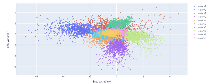
It's possible to obtain a better representation by applying the t-SNE, a dimensionality reduction method that converts the high dimensional input into two or three-dimensional data. In this case, I fix the number of components equal to 2, because I only need to do a bi-dimensional plot.

from sklearn.manifold import TSNE

tsne = TSNE(n_components=2)
tsne_results = tsne.fit_transform(encoded_samples.drop(['label'],axis=1))
fig = px.scatter(tsne_results, x=0, y=1,
				 color=encoded_samples.label.astype(str),
				 labels={'0': 'tsne-2d-one', '1': 'tsne-2d-two'})
fig.show()

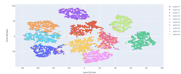
We can visualize a different cluster for each digit, except for some points falling into the wrong categories.

Final thoughts

Congratulations! You have learned to implement a Denoising autoencoder with convolutional layers. It's pretty easy to apply it when you already mastered the standard autoencoder. There are many other versions of autoencoders that can be tried, like the Variational Autoencoder and the Generative Additive Networks. The GitHub code is here. Thanks for reading. Have a nice day.