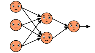
We understand that machine learning is about mapping inputs to targets. This is done by observing many examples of input and targets. We also know that deep neural networks do this input-to-target mapping via a deep sequence of simple data transformations. These are layers that these data transformations are learned by exposure to examples.
How this learning happens?
What a layer does to its input data specification is stored in the layer's weights. The layer's weights in essence are a bunch of numbers. We'd say that the transformation implemented by a layer is parameterized by its weights. Sometimes the weights are called parameters of layers. Learning have to means finding a set of values for the weights of all layers in a network. For instance, the network will correctly map example inputs to their associated targets.
A deep neural network may contain tens of millions of parameters. It is difficult task to find the correct value for all of them. To modify the value of one parameter will affect the behavior of all the others. First we need to be able to observe it,to control something. We need to be able to measure how far this output is from what we expected to control the output of a neural network.
Objective function
The objective function is the job of the loss function of the network. This is also called the objective function. The predictions are being taken by the loss function of the network and the true target. It computes a distance score, what we wanted the network to output by capturing how well the network has done on this specific example.
A basic trick in deep learning is to utilize this score as a feedback signal to adjust the value of the weights. This adjustment is the job of the optimizer. The optimizer implements what's called the Back propagation algorithm. It is the central algorithm in deep learning.
The weights of the network are assigned random values at the start. Therefore the network only implements a series of random transformations. Its output is away from what it should ideally be. The loss score is accordingly very high. The loss score decreases as the weights are adjusted a little in the correct direction. This training loop repeated a sufficient number of times.. This yields weight values that minimize the loss function.
Kernel methods
Kernel methods are a group of ,classification algorithms. These are best known to the support SVM vector machine. SVMs aim is to solve classification problems by finding good decision boundaries between two sets of points belonging to two different categories.
A decision boundary may be thought of as a line or surface separating our training data into two spaces corresponding to two categories. We just need to check which side of the decision boundary they fall on to classify new data points .SVMs proceed to find these boundaries in two steps:
- The data is mapped to a new high-dimensional representation where the decision boundary may be expressed as a hyperplane.
- A good decision boundary (a separation hyperplane) is computed by trying to maximize the distance between the hyperplane and the closest data points from each class.
This step is called maximizing the margin. This allows the boundary to generalize well to new samples outside of the training data set. A kernel function is a computationally tractable operation that maps any two points in our initial space to the distance between these points in our target representation space, completely bypassing the explicit computation of the new representation.
Typically, Kernel functions are crafted by hand rather than learned from data --- in the case of an SVM, only the separation hyperplane is learned. At the time they were developed, SVMs exhibited state-of-the-art performance on simple classification problems and were one of the few machine-learning methods backed by extensive theory and amenable to serious mathematical analysis, making them well understood and easily interpret able.
SVMs became extremely popular in the field for a long time due to these useful properties. SVMs are to be proved hard to scale to large datasets and didn't provide good results for perceptual problems such as image classification.
Applying an SVM to perceptual problems requires first extracting useful representations manually because an SVM is a shallow method that is difficult and brittle.
Decision trees
Decision trees let us classify input data points or predict output values given inputs. These are flowchart-like structures. They're easy to visualize and interpret.
Random Forest
This algorithm introduced a robust, practical take on decision-tree learning. It involves building a large number of specialized decision trees and then ensemble their outputs. Random forests are applicable to a big range of problems.
Gradient boosting machines
These are much like a random forest and is a machine-learning technique based on ensembling weak prediction models, generally decision trees.
Gradient boosting is being used that is a way to improve any machine-learning model by iteratively training new models that specialize in addressing the weak points of the previous models.
Applied to decision trees, the use of the gradient boosting technique results in models that strictly out perform random forests most of the time, while having similar proper-ties.
It may be one of the best algorithms for dealing with non perceptual data today. Alongside deep learning, it's one of the most commonly used techniques in Kaggle competitions.
Comments
Loading comments…